repository open issue

Contents

Hydroclimate Data Retriever

HyRiver (formerly named hydrodata) is a suite of Python packages that provides a unified API for retrieving geospatial/temporal data from various web services. HyRiver includes two categories of packages:

• Low-level APIs for accessing any of the supported web services, i.e., ArcGIS RESTful, WMS, and WFS.

• High-level APIs for accessing some of the most commonly used datasets in hyrdology and climatology studies. Currently, this project only includes hydrology and climatology data within the US.

You can watch these videos for a quick overview of HyRiver:

• Pangeo Showcase

• ESIP IT&I

Getting Started

Why HyRiver?

Some of the major capabilities of HyRiver are as follows:

• Easy access to many web services for subsetting data on server-side and returning the requests as masked Datasets or GeoDataFrames.

• Splitting large requests into smaller chunks, under-the-hood, since web services often limit the number of features per request. So the only bottleneck for subsetting the data is your local machine memory.

• Navigating and subsetting NHDPlus database (both medium- and high-resolution) using web services.

• Cleaning up the vector NHDPlus data, fixing some common issues, and computing vector-based accumulation through a river network.

• A URL inventory for some of the popular (and tested) web services.

• Some utilities for manipulating the obtained data and their visualization.

Installation

You can install all the packages using pip:

$ pip install py3dep pynhd pygeohydro pydaymet pygeoogc pygeoutils async_retriever

Please note that installation with pip fails if libgdal is not installed on your system. You should install this package manually beforehand. For example, on Ubuntu-based distros the required package is libgdal-dev. If this package is installed on your system you should be able to run gdal-config --version successfully.

Alternatively, you can use conda or mamba (recommended) to install these packages from the conda-forge repository:

$ conda install -c conda-forge py3dep pynhd pygeohydro pydaymet pygeoogc pygeoutils async_retriever

or:

$ mamba install -c conda-forge --strict-channel-priority py3dep pynhd pygeohydro pydaymet pygeoogc pygeoutils async_retriever

Dependencies

PyNHD

• async_retriever

• cytoolz

• geopandas

• networkx

• numpy

• pandas

• pyarrow

• pygeoogc

• pygeoutils

• requests

• shapely

• simplejson

PyGeoHydro

• async_retriever

• defusedxml

• folium

• geopandas

• lxml

• matplotlib

• numpy

• openpyxl

• pandas

• pygeoogc

• pygeoutils

• pynhd

• rasterio

• shapely

Py3DEP

• async_retriever

• click

• cytoolz

• numpy

• pydantic

• pygeoogc

• pygeoutils

• rasterio

• scipy

• shapely

• xarray

PyDaymet

• async_retriever

• click

• dask

• lxml

• numpy

• pandas

• py3dep

• pygeoogc

• pygeoutils

• rasterio

• scipy

• shapely

• xarray

PyGeoOGC

• async_retriever

• cytoolz

• defusedxml

• owslib

• pydantic

• pyproj

• pyyaml

• requests

• shapely

• simplejson

• urllib3

PyGeoUtils

• affine

• dask

• geopandas

• netcdf4

• numpy

• orjson

• pygeoogc

• pyproj

• rasterio

• shapely

• xarray

AsyncRetriever

• aiohttp-client-cache

• aiohttp[speedups]

• aiosqlite

• cytoolz

• nest-asyncio

• orjson

Additionally, you can also install bottleneck, pygeos, and rtree to improve performance of xarray and geopandas. For handling vector and raster data projections, cartopy and rioxarray are useful.

Software Stack

A detailed description of each component of the HyRiver software stack.

PyNHD

PyGeoHydro

Py3DEP

PyDaymet

AsyncRetriever

PyGeoOGC

PyGeoUtils

PyNHD: Navigate and subset NHDPlus database

Features

PyNHD is a part of HyRiver software stack that is designed to aid in watershed analysis through web services.

This package provides access to WaterData, the National Map’s NHDPlus HR, NLDI, and PyGeoAPI web services. These web services can be used to navigate and extract vector data from NHDPlus V2 (both medium- and high-resolution) database such as catchments, HUC8, HUC12, GagesII, flowlines, and water bodies. Moreover, PyNHD gives access to an item on ScienceBase called Select Attributes for NHDPlus Version 2.1 Reach Catchments and Modified Network Routed Upstream Watersheds for the Conterminous United States. This item provides over 30 attributes at catchment-scale based on NHDPlus ComIDs. These attributes are available in three categories:

1. Local (local): For individual reach catchments,

2. Total (upstream_acc): For network-accumulated values using total cumulative drainage area,

3. Divergence (div_routing): For network-accumulated values using divergence-routed.

Moreover, the PyGeoAPI service provides four functionalities:

1. flow_trace: Trace flow from a starting point to up/downstream direction.

2. split_catchment: Split the local catchment of a point of interest at the point’s location.

3. elevation_profile: Extract elevation profile along a flow path between two points.

4. cross_section: Extract cross-section at a point of interest along a flow line.

A list of these attributes for each characteristic type can be accessed using nhdplus_attrs function.

Similarly, PyNHD uses this item on Hydroshare to get ComID-linked NHDPlus Value Added Attributes. This dataset includes slope and roughness, among other attributes, for all the flowlines. You can use nhdplus_vaa function to get this dataset.

Additionally, PyNHD offers some extra utilities for processing the flowlines:

• prepare_nhdplus: For cleaning up the dataframe by, for example, removing tiny networks, adding a to_comid column, and finding a terminal flowlines if it doesn’t exist.

• topoogical_sort: For sorting the river network topologically which is useful for routing and flow accumulation.

• vector_accumulation: For computing flow accumulation in a river network. This function is generic, and any routing method can be plugged in.

These utilities are developed based on an R package called nhdplusTools.

All functions and classes that request data from web services use async_retriever that offers response caching. By default, the expiration time is set to never expire. All these functions and classes have two optional parameters for controlling the cache: expire_after and disable_caching. You can use expire_after to set the expiration time in seconds. If expire_after is set to -1, the cache will never expire (default). You can use disable_caching if you don’t want to use the cached responses. The cached responses are stored in the ./cache/aiohttp_cache.sqlite file.

You can find some example notebooks here.

Furthermore, you can try using PyNHD without even installing it on your system by clicking on the binder badge below the PyNHD banner. A JupyterLab instance with the software stack pre-installed and all example notebooks will be launched in your web browser, and you can start coding!

Please note that since this project is in early development stages, while the provided functionalities should be stable, changes in APIs are possible in new releases. But we appreciate it if you give this project a try and provide feedback. Contributions are most welcome.

Moreover, requests for additional functionalities can be submitted via issue tracker.

Installation

You can install PyNHD using pip after installing libgdal on your system (for example, in Ubuntu run sudo apt install libgdal-dev):

$ pip install pynhd

Alternatively, PyNHD can be installed from the conda-forge repository using Conda or Mamba:

$ conda install -c conda-forge pynhd

Quick start

Let’s explore the capabilities of NLDI. We need to instantiate the class first:

from pynhd import NLDI, WaterData, NHDPlusHR
import pynhd as nhd

First, let’s get the watershed geometry of the contributing basin of a USGS station using NLDI:

nldi = NLDI()
station_id = "01031500"

basin = nldi.get_basins(station_id)

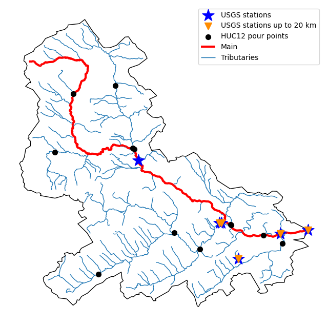
The navigate_byid class method can be used to navigate NHDPlus in both upstream and downstream of any point in the database. Let’s get ComIDs and flowlines of the tributaries and the main river channel in the upstream of the station.

flw_main = nldi.navigate_byid(
    fsource="nwissite",
    fid=f"USGS-{station_id}",
    navigation="upstreamMain",
    source="flowlines",
    distance=1000,
)

flw_trib = nldi.navigate_byid(
    fsource="nwissite",
    fid=f"USGS-{station_id}",
    navigation="upstreamTributaries",
    source="flowlines",
    distance=1000,
)

We can get other USGS stations upstream (or downstream) of the station and even set a distance limit (in km):

st_all = nldi.navigate_byid(
    fsource="nwissite",
    fid=f"USGS-{station_id}",
    navigation="upstreamTributaries",
    source="nwissite",
    distance=1000,
)

st_d20 = nldi.navigate_byid(
    fsource="nwissite",
    fid=f"USGS-{station_id}",
    navigation="upstreamTributaries",
    source="nwissite",
    distance=20,
)

Now, let’s get the HUC12 pour points:

pp = nldi.navigate_byid(
    fsource="nwissite",
    fid=f"USGS-{station_id}",
    navigation="upstreamTributaries",
    source="huc12pp",
    distance=1000,
)

Also, we can get the slope data for each river segment from NHDPlus VAA database:

vaa = nhd.nhdplus_vaa("input_data/nhdplus_vaa.parquet")

flw_trib["comid"] = pd.to_numeric(flw_trib.nhdplus_comid)
slope = gpd.GeoDataFrame(
    pd.merge(flw_trib, vaa[["comid", "slope"]], left_on="comid", right_on="comid"),
    crs=flw_trib.crs,
)
slope[slope.slope < 0] = np.nan

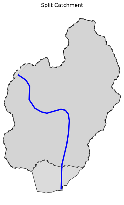
Now, let’s explore the PyGeoAPI capabilities:

pygeoapi = PyGeoAPI()

trace = pygeoapi.flow_trace(
    (1774209.63, 856381.68), crs="ESRI:102003", raindrop=False, direction="none"
)

split = pygeoapi.split_catchment((-73.82705, 43.29139), crs="epsg:4326", upstream=False)

profile = pygeoapi.elevation_profile(
    [(-103.801086, 40.26772), (-103.80097, 40.270568)], numpts=101, dem_res=1, crs="epsg:4326"
)

section = pygeoapi.cross_section((-103.80119, 40.2684), width=1000.0, numpts=101, crs="epsg:4326")

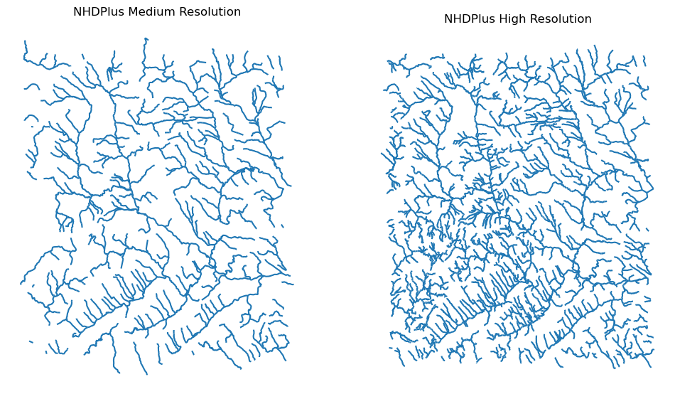
Next, we retrieve the medium- and high-resolution flowlines within the bounding box of our watershed and compare them. Moreover, Since several web services offer access to NHDPlus database, NHDPlusHR has an argument for selecting a service and also an argument for automatically switching between services.

mr = WaterData("nhdflowline_network")
nhdp_mr = mr.bybox(basin.geometry[0].bounds)

hr = NHDPlusHR("networknhdflowline", service="hydro", auto_switch=True)
nhdp_hr = hr.bygeom(basin.geometry[0].bounds)

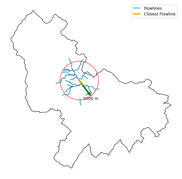
Moreover, WaterData can find features within a given radius (in meters) of a point:

eck4 = "+proj=eck4 +lon_0=0 +x_0=0 +y_0=0 +datum=WGS84 +units=m +no_defs"
coords = (-5727797.427596455, 5584066.49330473)
rad = 5e3
flw_rad = mr.bydistance(coords, rad, loc_crs=eck4)
flw_rad = flw_rad.to_crs(eck4)

Instead of getting all features within a radius of the coordinate, we can snap to the closest flowline using NLDI:

comid_closest = nldi.comid_byloc((x, y), eck4)
flw_closest = nhdp_mr.byid("comid", comid_closest.comid.values[0])

Since NHDPlus HR is still at the pre-release stage let’s use the MR flowlines to demonstrate the vector-based accumulation. Based on a topological sorted river network pynhd.vector_accumulation computes flow accumulation in the network. It returns a dataframe which is sorted from upstream to downstream that shows the accumulated flow in each node.

PyNHD has a utility called prepare_nhdplus that identifies such relationship among other things such as fixing some common issues with NHDPlus flowlines. But first we need to get all the NHDPlus attributes for each ComID since NLDI only provides the flowlines’ geometries and ComIDs which is useful for navigating the vector river network data. For getting the NHDPlus database we use WaterData. Let’s use the nhdflowline_network layer to get required info.

wd = WaterData("nhdflowline_network")

comids = flw_trib.nhdplus_comid.to_list()
nhdp_trib = wd.byid("comid", comids)
flw = nhd.prepare_nhdplus(nhdp_trib, 0, 0, purge_non_dendritic=False)

To demonstrate the use of routing, let’s use nhdplus_attrs function to get list of available NHDPlus attributes

char = "CAT_RECHG"
area = "areasqkm"

local = nldi.getcharacteristic_byid(comids, "local", char_ids=char)
flw = flw.merge(local[char], left_on="comid", right_index=True)


def runoff_acc(qin, q, a):
    return qin + q * a


flw_r = flw[["comid", "tocomid", char, area]]
runoff = nhd.vector_accumulation(flw_r, runoff_acc, char, [char, area])


def area_acc(ain, a):
    return ain + a


flw_a = flw[["comid", "tocomid", area]]
areasqkm = nhd.vector_accumulation(flw_a, area_acc, area, [area])

runoff /= areasqkm

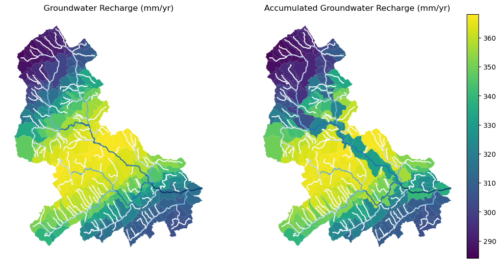
Since these are catchment-scale characteristic, let’s get the catchments then add the accumulated characteristic as a new column and plot the results.

wd = WaterData("catchmentsp")
catchments = wd.byid("featureid", comids)

c_local = catchments.merge(local, left_on="featureid", right_index=True)
c_acc = catchments.merge(runoff, left_on="featureid", right_index=True)

More examples can be found here.

PyGeoHydro: Retrieve Geospatial Hydrology Data

Features

PyGeoHydro (formerly named hydrodata) is a part of HyRiver software stack that is designed to aid in watershed analysis through web services. This package provides access to some public web services that offer geospatial hydrology data. It has three main modules: pygeohydro, plot, and helpers.

The pygeohydro module can pull data from the following web services:

• NWIS for daily mean streamflow observations (returned as a pandas.DataFrame or xarray.Dataset with station attributes),

• Water Quality Portal for accessing current and historical water quality data from more than 1.5 million sites across the US,

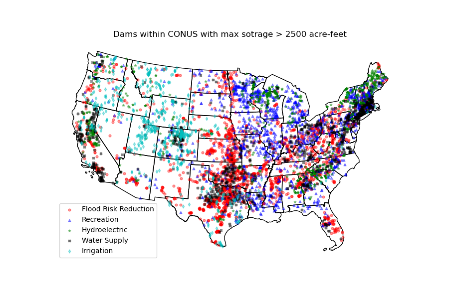
• NID for accessing the National Inventory of Dams web service,

• HCDN 2009 for identifying sites where human activity affects the natural flow of the watercourse,

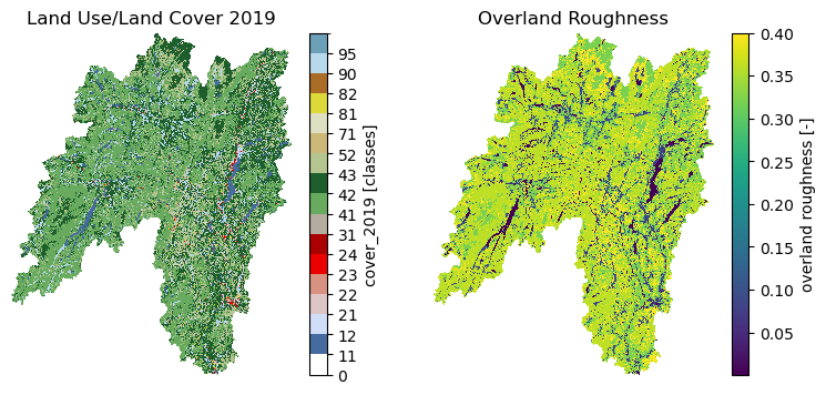
• NLCD 2019 for land cover/land use, imperviousness, imperviousness descriptor, and canopy data. You can get data using both geometries and coordinates.

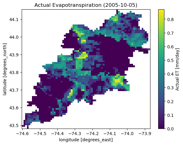
• SSEBop for daily actual evapotranspiration, for both single pixel and gridded data.

Also, it has two other functions:

• interactive_map: Interactive map for exploring NWIS stations within a bounding box.

• cover_statistics: Categorical statistics of land use/land cover data.

The plot module includes two main functions:

• signatures: Hydrologic signature graphs.

• cover_legends: Official NLCD land cover legends for plotting a land cover dataset.

• descriptor_legends: Color map and legends for plotting an imperviousness descriptor dataset.

The helpers module includes:

• nlcd_helper: A roughness coefficients lookup table for each land cover and imperviousness descriptor type which is useful for overland flow routing among other applications.

• nwis_error: A dataframe for finding information about NWIS requests’ errors.

Moreover, requests for additional databases and functionalities can be submitted via issue tracker.

You can find some example notebooks here.

You can also try using PyGeoHydro without installing it on your system by clicking on the binder badge. A Jupyter Lab instance with the HyRiver stack pre-installed will be launched in your web browser, and you can start coding!

Please note that since this project is in early development stages, while the provided functionalities should be stable, changes in APIs are possible in new releases. But we appreciate it if you give this project a try and provide feedback. Contributions are most welcome.

Moreover, requests for additional functionalities can be submitted via issue tracker.

Installation

You can install PyGeoHydro using pip after installing libgdal on your system (for example, in Ubuntu run sudo apt install libgdal-dev). Moreover, PyGeoHydro has an optional dependency for using persistent caching, requests-cache. We highly recommend installing this package as it can significantly speed up send/receive queries. You don’t have to change anything in your code, since PyGeoHydro under-the-hood looks for requests-cache and if available, it will automatically use persistent caching:

$ pip install pygeohydro

Alternatively, PyGeoHydro can be installed from the conda-forge repository using Conda:

$ conda install -c conda-forge pygeohydro

Quick start

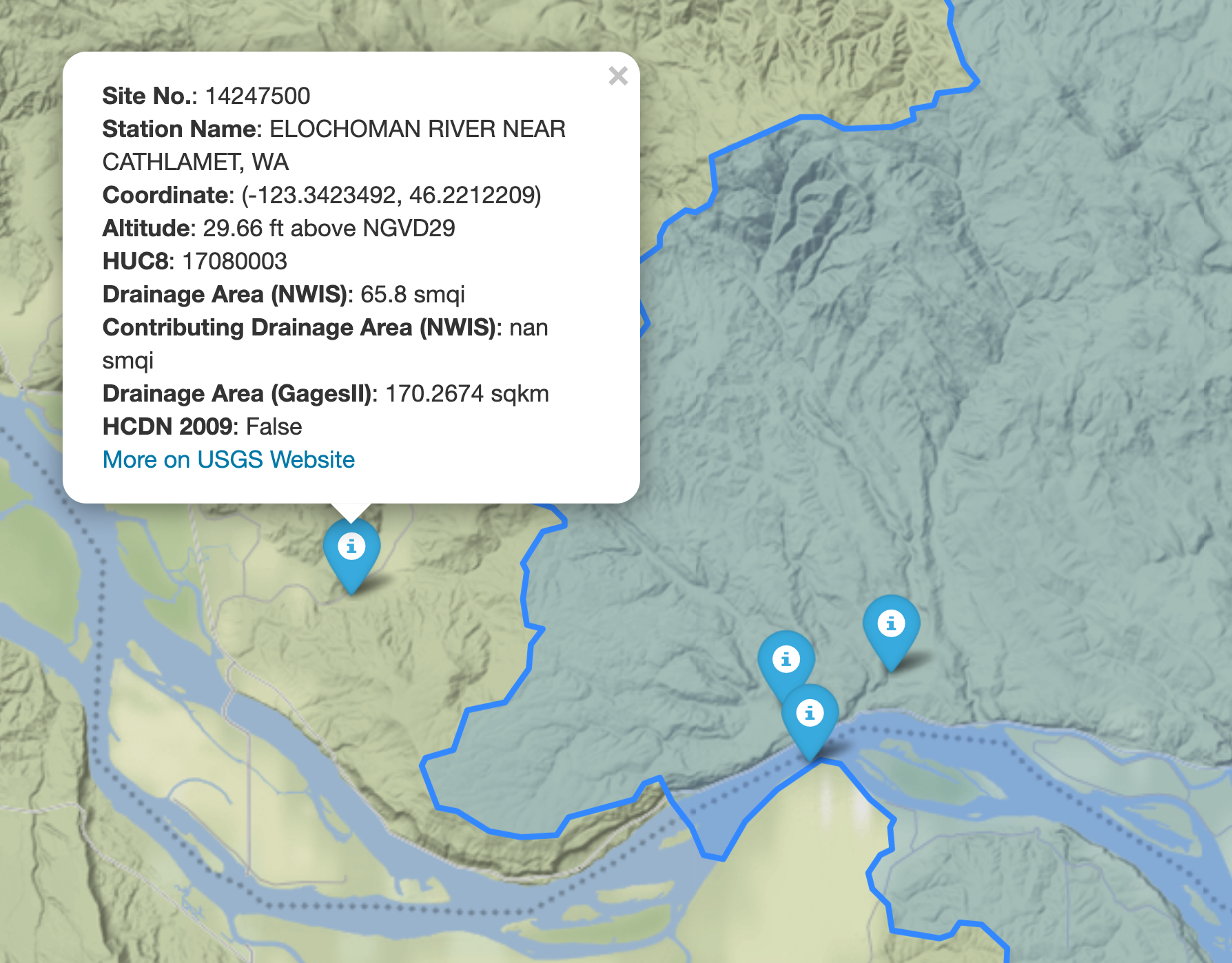
We can explore the available NWIS stations within a bounding box using interactive_map function. It returns an interactive map and by clicking on a station some of the most important properties of stations are shown.

import pygeohydro as gh

bbox = (-69.5, 45, -69, 45.5)
gh.interactive_map(bbox)

We can select all the stations within this boundary box that have daily mean streamflow data from 2000-01-01 to 2010-12-31:

from pygeohydro import NWIS

nwis = NWIS()
query = {
    **nwis.query_bybox(bbox),
    "hasDataTypeCd": "dv",
    "outputDataTypeCd": "dv",
}
info_box = nwis.get_info(query)
dates = ("2000-01-01", "2010-12-31")
stations = info_box[
    (info_box.begin_date <= dates[0]) & (info_box.end_date >= dates[1])
].site_no.tolist()

Then, we can get the daily streamflow data in mm/day (by default the values are in cms) and plot them:

from pygeohydro import plot

qobs = nwis.get_streamflow(stations, dates, mmd=True)
plot.signatures(qobs)

By default, get_streamflow returns a pandas.DataFrame that has a attrs method containing metadata for all the stations. You can access it like so qobs.attrs. Moreover, we can get the same data as xarray.Dataset as follows:

qobs_ds = nwis.get_streamflow(stations, dates, to_xarray=True)

This xarray.Dataset has two dimensions: time and station_id. It has 10 variables including discharge with two dimensions while other variables that are station attitudes are one dimensional.

We can also get instantaneous streamflow data using get_streamflow. This method assumes that the input dates are in UTC time zone and returns the data in UTC time zone as well.

date = ("2005-01-01 12:00", "2005-01-12 15:00")
qobs = nwis.get_streamflow("01646500", date, freq="iv")

The WaterQuality has a number of convenience methods to retrieve data from the web service. Since there are many parameter combinations that can be used to retrieve data, a general method is also provided to retrieve data from any of the valid endpoints. You can use get_json to retrieve stations info as a geopandas.GeoDataFrame or get_csv to retrieve stations data as a pandas.DataFrame. You can construct a dictionary of the parameters and pass it to one of these functions. For more information on the parameters, please consult the Water Quality Data documentation. For example, let’s find all the stations within a bounding box that have Caffeine data:

from pynhd import WaterQuality

bbox = (-92.8, 44.2, -88.9, 46.0)
kwds = {"characteristicName": "Caffeine"}
wq = WaterQuality()
stations = wq.station_bybbox(bbox, kwds)

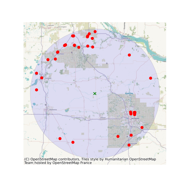
Or the same criterion but within a 30-mile radius of a point:

stations = wq.station_bydistance(-92.8, 44.2, 30, kwds)

Then we can get the data for all these stations the data like this:

sids = stations.MonitoringLocationIdentifier.tolist()
caff = wq.data_bystation(sids, kwds)

Moreover, we can get land use/land cove data using nlcd_bygeom or nlcd_bycoods functions and percentages of land cover types using cover_statistics. The nlcd_bycoords function returns a geopandas.GeoDataFrame with the NLCD layers as columns and input coordinates as the geometry column. Moreover, The nlcd_bygeom function accepts both a single geometry or a geopandas.GeoDataFrame as the input.

from pynhd import NLDI

basins = NLDI().get_basins(["01031450", "01031500", "01031510"])
lulc = gh.nlcd_bygeom(geometry, 100, years={"cover": [2016, 2019]})
stats = gh.cover_statistics(lulc.cover_2016)

Next, let’s use ssebopeta_bygeom to get actual ET data for a basin. Note that there’s a ssebopeta_bycoords function that returns an ETA time series for a single coordinate.

geometry = NLDI().get_basins("01315500").geometry[0]
eta = gh.ssebopeta_bygeom(geometry, dates=("2005-10-01", "2005-10-05"))

Additionally, we can pull all the US dams data using NID. Let’s get dams that are within this bounding box and have a maximum storage larger than 200 acre-feet.

nid = NID()
dams = nid.get_bygeom((-65.77, 43.07, -69.31, 45.45), "epsg:4326")
dams = nid.inventory_byid(dams.id.to_list())
dams = dams[dams.maxStorage > 200]

We can get also all dams within CONUS in NID with maximum storage larger than 200 acre-feet:

import geopandas as gpd

world = gpd.read_file(gpd.datasets.get_path("naturalearth_lowres"))
conus = world[world.name == "United States of America"].geometry.iloc[0].geoms[0]

dam_list = nid.get_byfilter([{"maxStorage": ["[200 5000]"]}])
dams = dam_list[0][dam_list[0].is_valid]
dams = dams[dams.within(conus)]

Py3DEP: Topographic data through 3DEP

Features

Py3DEP is a part of HyRiver software stack that is designed to aid in watershed analysis through web services. This package provides access to the 3DEP database which is a part of the National Map services. The 3DEP service has multi-resolution sources and depending on the user provided resolution, the data is resampled on the server-side based on all the available data sources. Py3DEP returns the requests as xarray dataset. Moreover, under-the-hood, this package uses requests-cache for persistent caching that can improve the performance significantly. The 3DEP web service includes the following layers:

• DEM

• Hillshade Gray

• Aspect Degrees

• Aspect Map

• GreyHillshade Elevation Fill

• Hillshade Multidirectional

• Slope Map

• Slope Degrees

• Hillshade Elevation Tinted

• Height Ellipsoidal

• Contour 25

• Contour Smoothed 25

Moreover, Py3DEP offers some additional utilities:

• elevation_bygrid: For getting elevations of all the grid points in a 2D grid.

• elevation_bycoords: For getting elevation of a list of x and y coordinates.

• deg2mpm: For converting slope dataset from degree to meter per meter.

You can try using Py3DEP without installing it on you system by clicking on the binder badge below the Py3DEP banner. A Jupyter notebook instance with the stack pre-installed will be launched in your web browser and you can start coding!

Please note that since this project is in early development stages, while the provided functionalities should be stable, changes in APIs are possible in new releases. But we appreciate it if you give this project a try and provide feedback. Contributions are most welcome.

Moreover, requests for additional functionalities can be submitted via issue tracker.

Installation

You can install Py3DEP using pip after installing libgdal on your system (for example, in Ubuntu run sudo apt install libgdal-dev). Moreover, Py3DEP has an optional dependency for using persistent caching, requests-cache. We highly recommend to install this package as it can significantly speedup send/receive queries. You don’t have to change anything in your code, since Py3DEP under-the-hood looks for requests-cache and if available, it will automatically use persistent caching:

$ pip install py3dep

Alternatively, Py3DEP can be installed from the conda-forge repository using Conda:

$ conda install -c conda-forge py3dep

Quick start

You can use Py3DEP using command-line or as a Python library. The commanda-line provides access to two functionality:

• Getting topographic data: You must create a geopandas.GeoDataFrame that contains the geometries of the target locations. This dataframe must have at least three columns: id, res, and geometry. The id column is used as filenames for saving the obtained topographic data to a NetCDF (.nc) file. The res column must be the target resolution in meter. Then, you must save the dataframe to a file with extensions such as .shp or .gpkg (whatever that geopandas.read_file can read).

• Getting elevation: You must create a pandas.DataFrame that contains coordinates of the target locations. This dataframe must have at least two columns: x and y. The elevations are obtained using airmap service in meters. The data are saved as a csv file with the same filename as the input file with an _elevation appended, e.g., coords_elevation.csv.

$ py3dep --help
Usage: py3dep [OPTIONS] COMMAND [ARGS]...

Command-line interface for Py3DEP.

Options:
-h, --help  Show this message and exit.

Commands:
coords    Retrieve topographic data for a list of coordinates.
geometry  Retrieve topographic data within geometries.

The coords sub-command is as follows:

$ py3dep coords -h
Usage: py3dep coords [OPTIONS] FPATH

Retrieve topographic data for a list of coordinates.

FPATH: Path to a csv file with two columns named ``lon`` and ``lat``.

Examples:
    $ cat coords.csv
    lon,lat
    -122.2493328,37.8122894
    $ py3dep coords coords.csv -q airmap -s topo_dir

Options:
-q, --query_source [airmap|tnm]
                                Source of the elevation data.
-s, --save_dir PATH             Path to a directory to save the requested
                                files. Extension for the outputs is either
                                `.nc` for geometry or `.csv` for coords.

-h, --help                      Show this message and exit.

And, the geometry sub-command is as follows:

$ py3dep geometry -h
Usage: py3dep geometry [OPTIONS] FPATH

Retrieve topographic data within geometries.

FPATH: Path to a shapefile (.shp) or geopackage (.gpkg) file.
This file must have three columns and contain a ``crs`` attribute:
    - ``id``: Feature identifiers that py3dep uses as the output netcdf/csv filenames.
    - ``res``: Target resolution in meters.
    - ``geometry``: A Polygon or MultiPloygon.

Examples:
    $ py3dep geometry ny_geom.gpkg -l "Slope Map" -l DEM -s topo_dir

Options:
-l, --layers [DEM|Hillshade Gray|Aspect Degrees|Aspect Map|GreyHillshade_elevationFill|Hillshade Multidirectional|Slope Map|Slope Degrees|Hillshade Elevation Tinted|Height Ellipsoidal|Contour 25|Contour Smoothed 25]
                                Target topographic data layers
-s, --save_dir PATH             Path to a directory to save the requested
                                files.Extension for the outputs is either
                                `.nc` for geometry or `.csv` for coords.

-h, --help                      Show this message and exit.

Now, let’s see how we can use Py3DEP as a library.

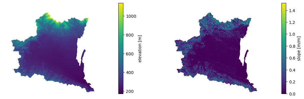
Py3DEP accepts Shapely’s Polygon or a bounding box (a tuple of length four) as an input geometry. We can use PyNHD to get a watershed’s geometry, then use it to get the DEM and slope in meters/meters from Py3DEP using get_map function.

The get_map has a resolution argument that sets the target resolution in meters. Note that the highest available resolution throughout the CONUS is about 10 m, though higher resolutions are available in limited parts of the US. Note that the input geometry can be in any valid spatial reference (geo_crs argument). The crs argument, however, is limited to CRS:84, EPSG:4326, and EPSG:3857 since 3DEP only supports these spatial references.

import py3dep
from pynhd import NLDI

geom = NLDI().get_basins("01031500").geometry[0]
dem = py3dep.get_map("DEM", geom, resolution=30, geo_crs="epsg:4326", crs="epsg:3857")
slope = py3dep.get_map("Slope Degrees", geom, resolution=30)
slope = py3dep.deg2mpm(slope)

We can use rioxarray package to save the obtained dataset as a raster file:

import rioxarray

dem.rio.to_raster("dem_01031500.tif")

Moreover, we can get the elevations of set of x- and y- coordinates on a grid. For example, let’s get the minimum temperature data within this watershed from Daymet using PyDaymet then add the elevation as a new variable to the dataset:

import pydaymet as daymet
import xarray as xr
import numpy as np

clm = daymet.get_bygeom(geometry, ("2005-01-01", "2005-01-31"), variables="tmin")
elev = py3dep.elevation_bygrid(clm.x.values, clm.y.values, clm.crs, clm.res[0] * 1000)
attrs = clm.attrs
clm = xr.merge([clm, elev])
clm["elevation"] = clm.elevation.where(~np.isnan(clm.isel(time=0).tmin), drop=True)
clm.attrs.update(attrs)

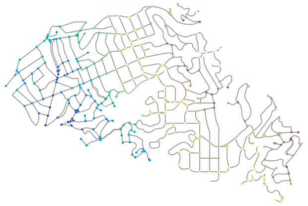
Now, let’s get street network data using osmnx package and add elevation data for its nodes using elevation_bycoords function.

import osmnx as ox

G = ox.graph_from_place("Piedmont, California, USA", network_type="drive")
x, y = nx.get_node_attributes(G, "x").values(), nx.get_node_attributes(G, "y").values()
elevation = py3dep.elevation_bycoords(zip(x, y), crs="epsg:4326")
nx.set_node_attributes(G, dict(zip(G.nodes(), elevation)), "elevation")

PyDaymet: Daily climate data through Daymet

Features

PyDaymet is a part of HyRiver software stack that is designed to aid in watershed analysis through web services. This package provides access to climate data from Daymet V4 database using NetCDF Subset Service (NCSS). Both single pixel (using get_bycoords function) and gridded data (using get_bygeom) are supported which are returned as pandas.DataFrame and xarray.Dataset, respectively. Climate data is available for North America, Hawaii from 1980, and Puerto Rico from 1950 at three time scales: daily, monthly, and annual. Additionally, PyDaymet can compute Potential EvapoTranspiration (PET) using three methods: penman_monteith, priestley_taylor, and hargreaves_samani for both single pixel and gridded data.

To fully utilize the capabilities of the NCSS, under-the-hood, PyDaymet uses AsyncRetriever for retrieving Daymet data asynchronously with persistent caching. This improves the reliability and speed of data retrieval significantly.

You can try using PyDaymet without installing it on you system by clicking on the binder badge below the PyDaymet banner. A Jupyter notebook instance with the stack pre-installed will be launched in your web browser and you can start coding!

Please note that since this project is in early development stages, while the provided functionalities should be stable, changes in APIs are possible in new releases. But we appreciate it if you give this project a try and provide feedback. Contributions are most welcome.

Moreover, requests for additional functionalities can be submitted via issue tracker.

Installation

You can install PyDaymet using pip after installing libgdal on your system (for example, in Ubuntu run sudo apt install libgdal-dev):

$ pip install pydaymet

Alternatively, PyDaymet can be installed from the conda-forge repository using Conda:

$ conda install -c conda-forge pydaymet

Quick start

You can use PyDaymet using command-line or as a Python library. The commanda-line provides access to two functionality:

• Getting gridded climate data: You must create a geopandas.GeoDataFrame that contains the geometries of the target locations. This dataframe must have four columns: id, start, end, geometry. The id column is used as filenames for saving the obtained climate data to a NetCDF (.nc) file. The start and end columns are starting and ending dates of the target period. Then, you must save the dataframe as a shapefile (.shp) or geopackage (.gpkg) with CRS attribute.

• Getting single pixel climate data: You must create a CSV file that contains coordinates of the target locations. This file must have at four columns: id, start, end, lon, and lat. The id column is used as filenames for saving the obtained climate data to a CSV (.csv) file. The start and end columns are the same as the geometry command. The lon and lat columns are the longitude and latitude coordinates of the target locations.

$ pydaymet -h
Usage: pydaymet [OPTIONS] COMMAND [ARGS]...

Command-line interface for PyDaymet.

Options:
-h, --help  Show this message and exit.

Commands:
coords    Retrieve climate data for a list of coordinates.
geometry  Retrieve climate data for a dataframe of geometries.

The coords sub-command is as follows:

$ pydaymet coords -h
Usage: pydaymet coords [OPTIONS] FPATH

Retrieve climate data for a list of coordinates.

FPATH: Path to a csv file with four columns:
    - ``id``: Feature identifiers that daymet uses as the output netcdf filenames.
    - ``start``: Start time.
    - ``end``: End time.
    - ``lon``: Longitude of the points of interest.
    - ``lat``: Latitude of the points of interest.
    - ``time_scale``: (optional) Time scale, either ``daily`` (default), ``monthly`` or ``annual``.
    - ``pet``: (optional) Method to compute PET. Suppoerted methods are:
               ``penman_monteith``, ``hargreaves_samani``, ``priestley_taylor``, and ``none`` (default).
    - ``alpha``: (optional) Alpha parameter for Priestley-Taylor method for computing PET. Defaults to 1.26.

Examples:
    $ cat coords.csv
    id,lon,lat,start,end,pet
    california,-122.2493328,37.8122894,2012-01-01,2014-12-31,hargreaves_samani
    $ pydaymet coords coords.csv -v prcp -v tmin

Options:
-v, --variables TEXT  Target variables. You can pass this flag multiple
                        times for multiple variables.

-s, --save_dir PATH   Path to a directory to save the requested files.
                        Extension for the outputs is .nc for geometry and .csv
                        for coords.

-h, --help            Show this message and exit.

And, the geometry sub-command is as follows:

$ pydaymet geometry -h
Usage: pydaymet geometry [OPTIONS] FPATH

Retrieve climate data for a dataframe of geometries.

FPATH: Path to a shapefile (.shp) or geopackage (.gpkg) file.
This file must have four columns and contain a ``crs`` attribute:
    - ``id``: Feature identifiers that daymet uses as the output netcdf filenames.
    - ``start``: Start time.
    - ``end``: End time.
    - ``geometry``: Target geometries.
    - ``time_scale``: (optional) Time scale, either ``daily`` (default), ``monthly`` or ``annual``.
    - ``pet``: (optional) Method to compute PET. Suppoerted methods are:
               ``penman_monteith``, ``hargreaves_samani``, ``priestley_taylor``, and ``none`` (default).
    - ``alpha``: (optional) Alpha parameter for Priestley-Taylor method for computing PET. Defaults to 1.26.

Examples:
    $ pydaymet geometry geo.gpkg -v prcp -v tmin

Options:
-v, --variables TEXT  Target variables. You can pass this flag multiple
                        times for multiple variables.

-s, --save_dir PATH   Path to a directory to save the requested files.
                        Extension for the outputs is .nc for geometry and .csv
                        for coords.

-h, --help            Show this message and exit.

Now, let’s see how we can use PyDaymet as a library.

PyDaymet offers two functions for getting climate data; get_bycoords and get_bygeom. The arguments of these functions are identical except the first argument where the latter should be polygon and the former should be a coordinate (a tuple of length two as in (x, y)). The input geometry or coordinate can be in any valid CRS (defaults to EPSG:4326). The dates argument can be either a tuple of length two like (start_str, end_str) or a list of years like [2000, 2005]. It is noted that both functions have a pet flag for computing PET. Additionally, we can pass time_scale to get daily, monthly or annual summaries. This flag by default is set to daily.

from pynhd import NLDI
import pydaymet as daymet

geometry = NLDI().get_basins("01031500").geometry[0]

var = ["prcp", "tmin"]
dates = ("2000-01-01", "2000-06-30")

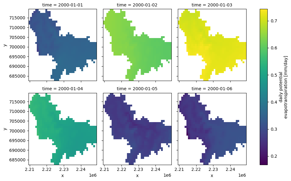
daily = daymet.get_bygeom(geometry, dates, variables=var, pet="priestley_taylor")
monthly = daymet.get_bygeom(geometry, dates, variables=var, time_scale="monthly")

If the input geometry (or coordinate) is in a CRS other than EPSG:4326, we should pass it to the functions.

coords = (-1431147.7928, 318483.4618)
crs = "epsg:3542"
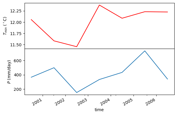
dates = ("2000-01-01", "2006-12-31")
annual = daymet.get_bycoords(coords, dates, variables=var, loc_crs=crs, time_scale="annual")

Also, we can use the potential_et function to compute PET by passing the daily climate data. We can either pass a pandas.DataFrame or a xarray.Dataset. Note that, penman_monteith and priestley_taylor methods have parameters that can be passed via the params argument, if any value other than the default values are needed. For example, default value of alpha for priestley_taylor method is 1.26 (humid regions), we can set it to 1.74 (arid regions) as follows:

pet_hs = daymet.potential_et(daily, methods="priestley_taylor", params={"alpha": 1.74})

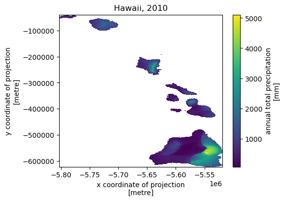
Next, let’s get annual total precipitation for Hawaii and Puerto Rico for 2010.

hi_ext = (-160.3055, 17.9539, -154.7715, 23.5186)
pr_ext = (-67.9927, 16.8443, -64.1195, 19.9381)
hi = daymet.get_bygeom(hi_ext, 2010, variables="prcp", region="hi", time_scale="annual")
pr = daymet.get_bygeom(pr_ext, 2010, variables="prcp", region="pr", time_scale="annual")

Some example plots are shown below:

AsyncRetriever: Asynchronous requests with persistent caching

Features

AsyncRetriever is a part of HyRiver software stack that is designed to aid in watershed analysis through web services. This package has only one purpose; asynchronously sending requests and retrieving responses as text, binary, or json objects. It uses persistent caching to speed up the retrieval even further. Moreover, thanks to nest_asyncio you can use this package in Jupyter notebooks. Although this package is in the HyRiver software stack, it’s applicable to any HTTP requests.

Please note that since this project is in early development stages, while the provided functionalities should be stable, changes in APIs are possible in new releases. But we appreciate it if you give this project a try and provide feedback. Contributions are most welcome.

Moreover, requests for additional functionalities can be submitted via issue tracker.

Installation

You can install async_retriever using pip:

$ pip install async_retriever

Alternatively, async_retriever can be installed from the conda-forge repository using Conda:

$ conda install -c conda-forge async_retriever

Quick start

AsyncRetriever has two public function: retrieve for sending requests and delete_url_cache for removing all requests from the cache file that contain a given URL. By default, retrieve creates and/or uses ./cache/aiohttp_cache.sqlite as the cache that you can customize it by the cache_name argument. Also, by default, the cache doesn’t have any expiration date and the delete_url_cache function should be used if you know that a database on a server was updated, and you want to retrieve the latest data. Alternatively, you can use the expire_after argument to set the expiration date for the cache.

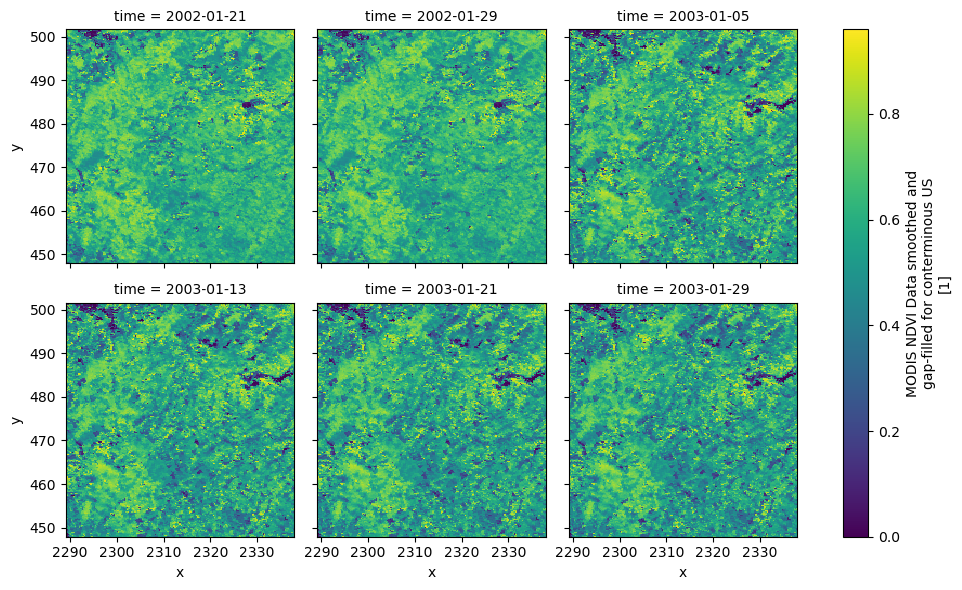
As an example for retrieving a binary response, let’s use the DAAC server to get NDVI. The responses can be directly passed to xarray.open_mfdataset to get the data as a xarray Dataset. We can also disable SSL certificate verification by setting ssl=False.

import io
import xarray as xr
import async_retriever as ar
from datetime import datetime

west, south, east, north = (-69.77, 45.07, -69.31, 45.45)
base_url = "https://thredds.daac.ornl.gov/thredds/ncss/ornldaac/1299"
dates_itr = ((datetime(y, 1, 1), datetime(y, 1, 31)) for y in range(2000, 2005))
urls, kwds = zip(
    *[
        (
            f"{base_url}/MCD13.A{s.year}.unaccum.nc4",
            {
                "params": {
                    "var": "NDVI",
                    "north": f"{north}",
                    "west": f"{west}",
                    "east": f"{east}",
                    "south": f"{south}",
                    "disableProjSubset": "on",
                    "horizStride": "1",
                    "time_start": s.strftime("%Y-%m-%dT%H:%M:%SZ"),
                    "time_end": e.strftime("%Y-%m-%dT%H:%M:%SZ"),
                    "timeStride": "1",
                    "addLatLon": "true",
                    "accept": "netcdf",
                }
            },
        )
        for s, e in dates_itr
    ]
)
resp = ar.retrieve(urls, "binary", request_kwds=kwds, max_workers=8, ssl=False)
data = xr.open_mfdataset(io.BytesIO(r) for r in resp)

We can remove these requests and their responses from the cache like so:

ar.delete_url_cache(base_url)

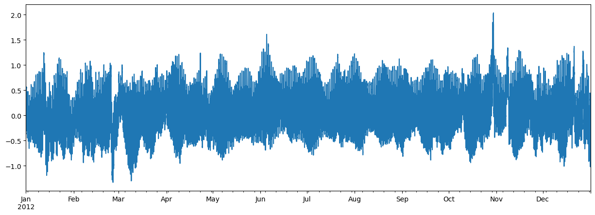
For a json response example, let’s get water level recordings of a NOAA’s water level station, 8534720 (Atlantic City, NJ), during 2012, using CO-OPS API. Note that this CO-OPS product has a 31-day limit for a single request, so we have to break the request down accordingly.

import pandas as pd

station_id = "8534720"
start = pd.to_datetime("2012-01-01")
end = pd.to_datetime("2012-12-31")

s = start
dates = []
for e in pd.date_range(start, end, freq="m"):
    dates.append((s.date(), e.date()))
    s = e + pd.offsets.MonthBegin()

url = "https://api.tidesandcurrents.noaa.gov/api/prod/datagetter"

urls, kwds = zip(
    *[
        (
            url,
            {
                "params": {
                    "product": "water_level",
                    "application": "web_services",
                    "begin_date": f'{s.strftime("%Y%m%d")}',
                    "end_date": f'{e.strftime("%Y%m%d")}',
                    "datum": "MSL",
                    "station": f"{station_id}",
                    "time_zone": "GMT",
                    "units": "metric",
                    "format": "json",
                }
            },
        )
        for s, e in dates
    ]
)

resp = ar.retrieve(urls, read="json", request_kwds=kwds, cache_name="~/.cache/async.sqlite")
wl_list = []
for rjson in resp:
    wl = pd.DataFrame.from_dict(rjson["data"])
    wl["t"] = pd.to_datetime(wl.t)
    wl = wl.set_index(wl.t).drop(columns="t")
    wl["v"] = pd.to_numeric(wl.v, errors="coerce")
    wl_list.append(wl)
water_level = pd.concat(wl_list).sort_index()
water_level.attrs = rjson["metadata"]

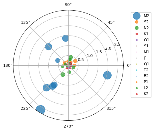
Now, let’s see an example without any payload or headers. Here’s how we can retrieve harmonic constituents of several NOAA stations from CO-OPS:

stations = [
    "8410140",
    "8411060",
    "8413320",
    "8418150",
    "8419317",
    "8419870",
    "8443970",
    "8447386",
]

base_url = "https://api.tidesandcurrents.noaa.gov/mdapi/prod/webapi/stations"
urls = [f"{base_url}/{i}/harcon.json?units=metric" for i in stations]
resp = ar.retrieve(urls, "json")

amp_list = []
phs_list = []
for rjson in resp:
    sid = rjson["self"].rsplit("/", 2)[1]
    const = pd.DataFrame.from_dict(rjson["HarmonicConstituents"]).set_index("name")
    amp = const.rename(columns={"amplitude": sid})[sid]
    phase = const.rename(columns={"phase_GMT": sid})[sid]
    amp_list.append(amp)
    phs_list.append(phase)

amp = pd.concat(amp_list, axis=1)
phs = pd.concat(phs_list, axis=1)

PyGeoOGC: Retrieve Data from RESTful, WMS, and WFS Services

Features

PyGeoOGC is a part of HyRiver software stack that is designed to aid in watershed analysis through web services. This package provides general interfaces to web services that are based on ArcGIS RESTful, WMS, and WFS. Although all these web service have limits on the number of features per requests (e.g., 1000 object IDs for a RESTful request or 8 million pixels for a WMS request), PyGeoOGC divides requests into smaller chunks, under-the-hood, and then merges the results.

All functions and classes that request data from web services use async_retriever that offers response caching. By default, the expiration time is set to never expire. All these functions and classes have two optional parameters for controlling the cache: expire_after and disable_caching. You can use expire_after to set the expiration time in seconds. If expire_after is set to -1, the cache will never expire (default). You can use disable_caching if you don’t want to use the cached responses. The cached responses are stored in the ./cache/aiohttp_cache.sqlite file.

There is also an inventory of URLs for some of these web services in form of a class called ServiceURL. These URLs are in four categories: ServiceURL().restful, ServiceURL().wms, ServiceURL().wfs, and ServiceURL().http. These URLs provide you with some examples of the services that PyGeoOGC supports. All the URLs are read from a YAML file located here. If you have success using PyGeoOGC with a web service please consider submitting a request to be added to this URL inventory, located at pygeoogc/static/urls.yml.

PyGeoOGC has three main classes:

• ArcGISRESTful: This class can be instantiated by providing the target layer URL. For example, for getting Watershed Boundary Data we can use ServiceURL().restful.wbd. By looking at the web service’s website we see that there are nine layers. For example, 1 for 2-digit HU (Region), 6 for 12-digit HU (Subregion), and so on. We can pass the URL to the target layer directly, like this f"{ServiceURL().restful.wbd}/6" or as a separate argument via layer.

  Afterward, we request for the data in two steps. First, we need to get the target object IDs using oids_bygeom (within a geometry), oids_byfield (specific field IDs), or oids_bysql (any valid SQL 92 WHERE clause) class methods. Then, we can get the target features using get_features class method. The returned response can be converted into a GeoDataFrame using json2geodf function from PyGeoUtils.

• WMS: Instantiation of this class requires at least 3 arguments: service URL, layer name(s), and output format. Additionally, target CRS and the web service version can be provided. Upon instantiation, we can use getmap_bybox method class to get the target raster data within a bounding box. The box can be in any valid CRS and if it is different from the default CRS, EPSG:4326, it should be passed using box_crs argument. The service response can be converted into a xarray.Dataset using gtiff2xarray function from PyGeoUtils.

• WFS: Instantiation of this class is similar to WMS. The only difference is that only one layer name can be passed. Upon instantiation there are three ways to get the data:

  • getfeature_bybox: Get all the target features within a bounding box in any valid CRS.

  • getfeature_byid: Get all the target features based on the IDs. Note that two arguments should be provided: featurename, and featureids. You can get a list of valid feature names using get_validnames class method.

  • getfeature_byfilter: Get the data based on any valid CQL filter.

  You can convert the returned response of this function to a GeoDataFrame using json2geodf function from PyGeoUtils package.

You can find some example notebooks here.

Furthermore, you can try using PyGeoOGC without even installing it on your system by clicking on the binder badge below the PyGeoOGC banner. A JupyterLab instance with the software stack pre-installed and all example notebooks will be launched in your web browser, and you can start coding!

Please note that since this project is in early development stages, while the provided functionalities should be stable, changes in APIs are possible in new releases. But we appreciate it if you give this project a try and provide feedback. Contributions are most welcome.

Moreover, requests for additional functionalities can be submitted via issue tracker.

Installation

You can install PyGeoOGC using pip:

$ pip install pygeoogc

Alternatively, PyGeoOGC can be installed from the conda-forge repository using Conda or Mamba:

$ conda install -c conda-forge pygeoogc

Quick start

We can access NHDPlus HR via RESTful service, National Wetlands Inventory from WMS, and FEMA National Flood Hazard via WFS. The output for these functions are of type requests.Response that can be converted to GeoDataFrame or xarray.Dataset using PyGeoUtils.

Let’s start the National Map’s NHDPlus HR web service. We can query the flowlines that are within a geometry as follows:

from pygeoogc import ArcGISRESTful, WFS, WMS, ServiceURL
import pygeoutils as geoutils
from pynhd import NLDI

basin_geom = NLDI().get_basins("01031500").geometry[0]

hr = ArcGISRESTful(ServiceURL().restful.nhdplushr, 2, outformat="json")

resp = hr.get_features(hr.oids_bygeom(basin_geom, "epsg:4326"))
flowlines = geoutils.json2geodf(resp)

Note oids_bygeom has three additional arguments: sql_clause, spatial_relation, and distance. We can use sql_clause for passing any valid SQL WHERE clauses and spatial_relation for specifying the target predicate such as intersect, contain, cross, etc. The default predicate is intersect (esriSpatialRelIntersects). Additionally, we can use distance for specifying the buffer distance from the input geometry for getting features.

We can also submit a query based on IDs of any valid field in the database. If the measure property is desired you can pass return_m as True to the get_features class method:

oids = hr.oids_byfield("PERMANENT_IDENTIFIER", ["103455178", "103454362", "103453218"])
resp = hr.get_features(oids, return_m=True)
flowlines = geoutils.json2geodf(resp)

Additionally, any valid SQL 92 WHERE clause can be used. For more details look here. For example, let’s limit our first request to only include catchments with areas larger than 0.5 sqkm.

oids = hr.oids_bygeom(basin_geom, geo_crs="epsg:4326", sql_clause="AREASQKM > 0.5")
resp = hr.get_features(oids)
catchments = geoutils.json2geodf(resp)

A WMS-based example is shown below:

wms = WMS(
    ServiceURL().wms.fws,
    layers="0",
    outformat="image/tiff",
    crs="epsg:3857",
)
r_dict = wms.getmap_bybox(
    basin_geom.bounds,
    1e3,
    box_crs="epsg:4326",
)
wetlands = geoutils.gtiff2xarray(r_dict, basin_geom, "epsg:4326")

Query from a WFS-based web service can be done either within a bounding box or using any valid CQL filter.

wfs = WFS(
    ServiceURL().wfs.fema,
    layer="public_NFHL:Base_Flood_Elevations",
    outformat="esrigeojson",
    crs="epsg:4269",
)
r = wfs.getfeature_bybox(basin_geom.bounds, box_crs="epsg:4326")
flood = geoutils.json2geodf(r.json(), "epsg:4269", "epsg:4326")

layer = "wmadata:huc08"
wfs = WFS(
    ServiceURL().wfs.waterdata,
    layer=layer,
    outformat="application/json",
    version="2.0.0",
    crs="epsg:4269",
)
r = wfs.getfeature_byfilter(f"huc8 LIKE '13030%'")
huc8 = geoutils.json2geodf(r.json(), "epsg:4269", "epsg:4326")

PyGeoUtils: Utilities for (Geo)JSON and (Geo)TIFF Conversion

Features

PyGeoUtils is a part of HyRiver software stack that is designed to aid in watershed analysis through web services. This package provides utilities for manipulating (Geo)JSON and (Geo)TIFF responses from web services. These utilities are:

• json2geodf: For converting (Geo)JSON objects to GeoPandas dataframe.

• arcgis2geojson: For converting ESRIGeoJSON to the standard GeoJSON format.

• gtiff2xarray: For converting (Geo)TIFF objects to xarray. datasets.

• xarray2geodf: For converting xarray.DataArray to a geopandas.GeoDataFrame, i.e., vectorization.

• xarray_geomask: For masking a xarray.Dataset or xarray.DataArray using a polygon.

All these functions handle all necessary CRS transformations.

You can find some example notebooks here.

Please note that since this project is in early development stages, while the provided functionalities should be stable, changes in APIs are possible in new releases. But we appreciate it if you give this project a try and provide feedback. Contributions are most welcome.

Moreover, requests for additional functionalities can be submitted via issue tracker.

Installation

You can install PyGeoUtils using pip after installing libgdal on your system (for example, in Ubuntu run sudo apt install libgdal-dev). Moreover, PyGeoUtils has an optional dependency for using persistent caching, requests-cache. We highly recommend to install this package as it can significantly speedup send/receive queries. You don’t have to change anything in your code, since PyGeoUtils under-the-hood looks for requests-cache and if available, it will automatically use persistent caching:

$ pip install pygeoutils

Alternatively, PyGeoUtils can be installed from the conda-forge repository using Conda:

$ conda install -c conda-forge pygeoutils

Quick start

To demonstrate capabilities of PyGeoUtils let’s use PyGeoOGC to access National Wetlands Inventory from WMS, and FEMA National Flood Hazard via WFS, then convert the output to xarray.Dataset and GeoDataFrame, respectively.

import pygeoutils as geoutils
from pygeoogc import WFS, WMS, ServiceURL
from shapely.geometry import Polygon


geometry = Polygon(
    [
        [-118.72, 34.118],
        [-118.31, 34.118],
        [-118.31, 34.518],
        [-118.72, 34.518],
        [-118.72, 34.118],
    ]
)
crs = "epsg:4326"

wms = WMS(
    ServiceURL().wms.mrlc,
    layers="NLCD_2011_Tree_Canopy_L48",
    outformat="image/geotiff",
    crs=crs,
)
r_dict = wms.getmap_bybox(
    geometry.bounds,
    1e3,
    box_crs=crs,
)
canopy = geoutils.gtiff2xarray(r_dict, geometry, crs)

mask = canopy > 60
canopy_gdf = geoutils.xarray2geodf(canopy, "float32", mask)

url_wfs = "https://hazards.fema.gov/gis/nfhl/services/public/NFHL/MapServer/WFSServer"
wfs = WFS(
    url_wfs,
    layer="public_NFHL:Base_Flood_Elevations",
    outformat="esrigeojson",
    crs="epsg:4269",
)
r = wfs.getfeature_bybox(geometry.bounds, box_crs=crs)
flood = geoutils.json2geodf(r.json(), "epsg:4269", crs)

Example Gallery

The following notebooks demonstrate capabilities of the HyRiver software stack.

This page was generated from notebooks/3dep.ipynb. Interactive online version:

Topographic Data

from pathlib import Path

import matplotlib.pyplot as plt
import networkx as nx
import numpy as np
import osmnx as ox
import py3dep
import pydaymet as daymet
import rioxarray  # noqa: F401
import xarray as xr
from pynhd import NLDI

Py3DEP provides access to the 3DEP database which is a part of the National Map services. The 3DEP service has multi-resolution sources and depending on the user provided resolution, the data is resampled on the server-side based on all the available data sources. Py3DEP returns the requests as xarray dataset. The 3DEP includes the following layers:

• DEM

• Hillshade Gray

• Aspect Degrees

• Aspect Map

• GreyHillshade Elevation Fill

• Hillshade Multidirectional

• Slope Map

• Slope Degrees

• Hillshade Elevation Tinted

• Height Ellipsoidal

• Contour 25

• Contour Smoothed 25

Moreover, Py3DEP offers some additional utilities:

• elevation_bygrid: For getting elevations of all the grid points in a 2D grid.

• elevation_byloc: For getting elevation of a single point which is based on the National Map’s Elevation Point Query Service.

• deg2mpm: For converting slope dataset from degree to meter per meter.

Let’s get a watershed geometry using NLDI and then get DEM and slope.

geometry = NLDI().get_basins("11092450").geometry[0]

dem = py3dep.get_map("DEM", geometry, resolution=90, geo_crs="epsg:4326", crs="epsg:3857")
dem.name = "dem"
dem.attrs["units"] = "meters"
slope = py3dep.get_map("Slope Degrees", geometry, resolution=30)
slope = py3dep.deg2mpm(slope)

We can save the DEM DataArray as a raster file using rioxarray:

dem.rio.to_raster(Path("input_data", "dem_11092450.tif"))

fig, (ax1, ax2) = plt.subplots(nrows=1, ncols=2, figsize=(15, 5))
dem.plot(ax=ax1)
slope.plot(ax=ax2)
fig.savefig("_static/dem_slope.png", bbox_inches="tight", facecolor="w")

We can also get elevations of a list of coordinates using py3dep.elevation_bycoords function. This function is particularly useful for getting elevations of nodes of a network, for example, is a river or a street network. Let’s use osmnx package to get a street network:

G = ox.graph_from_place("Piedmont, California, USA", network_type="drive")

Now, we can get the elevations for each node based on their coordinates and then plot the results.

x, y = nx.get_node_attributes(G, "x").values(), nx.get_node_attributes(G, "y").values()
elevation = py3dep.elevation_bycoords(list(zip(x, y)), crs="epsg:4326")
nx.set_node_attributes(G, dict(zip(G.nodes(), elevation)), "elevation")

nc = ox.plot.get_node_colors_by_attr(G, "elevation", cmap="terrain")
fig, ax = ox.plot_graph(
    G,
    node_color=nc,
    node_size=10,
    save=True,
    bgcolor="w",
    filepath="_static/street_elev.png",
    dpi=100,
)

Note that, this function gets the elevation data from the elevation map of the bounding box of all the coordinates. So, if the larger the extent of this bounding box, the longer is going to take for the function to get the data.

Additionally, we can get the elevations of set of x- and y- coordinates of a grid. For example, let’s get the minimum temperature data within the watershed from Daymet using PyDaymet then add the elevation as a new variable to the dataset:

clm = daymet.get_bygeom(geometry, ("2005-01-01", "2005-01-31"), variables="tmin")
elev = py3dep.elevation_bygrid(clm.x.values, clm.y.values, clm.crs, clm.res[0] * 1000)
attrs = clm.attrs
clm = xr.merge([clm, elev])
clm["elevation"] = clm.elevation.where(~np.isnan(clm.isel(time=0).tmin), drop=True)
clm.attrs.update(attrs)

fig, (ax1, ax2) = plt.subplots(nrows=1, ncols=2, figsize=(15, 5))
clm.tmin.isel(time=10).plot(ax=ax1)
clm.elevation.plot(ax=ax2)

<matplotlib.collections.QuadMesh at 0x1ab50c8b0>

This page was generated from notebooks/aridity.ipynb. Interactive online version:

Aridity

PyDaymet computes Potential Evaportranspiration based on FAO Penman-Monteith equation using tmin (deg c), tmax (deg c), vp (Pa), srad (W/m^2), and dayl (s) variables from Daymet:

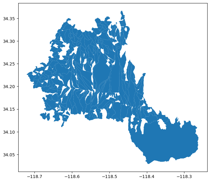
Basin

Let’s start by getting the basin geometry of USGS-01031500 station (Piscataquis River near Dover-Foxcroft, Maine)

import os
import warnings
from pathlib import Path

import geopandas as gpd
import pynhd as nhd

warnings.filterwarnings("ignore", message=".*initial implementation of Parquet.*")
root = Path("input_data")
os.makedirs(root, exist_ok=True)
BASE_PLOT = {"facecolor": "k", "edgecolor": "b", "alpha": 0.2, "figsize": (18, 9)}
CRS = "esri:102008"
station_id = "01031500"

nldi = nhd.NLDI()
cfile = Path(root, f"basin_{station_id}.feather")
if cfile.exists():
    basin = gpd.read_feather(cfile)
else:
    basin = nldi.get_basins(station_id)
    basin.to_feather(cfile)

ax = basin.to_crs(CRS).plot(**BASE_PLOT)
ax.axis("off")
ax.margins(0)

Precipitation and Potential Evapotranspiration

import pydaymet as daymet
from tqdm.notebook import tqdm

years = list(range(2006, 2016))
geometry = basin.iloc[0].geometry

for yr in tqdm(years, desc="Getting Climate"):
    cfile = Path(root, f"clm_{yr}.nc")
    if cfile.exists():
        continue
    daymet.get_bygeom(geometry, yr, variables="prcp", pet="hargreaves_samani").to_netcdf(cfile)

import xarray as xr

clm = xr.open_mfdataset(Path(root).glob("clm_*.nc"), coords="minimal")
clm["elevation"] = clm["elevation"].isel(time=0, drop=True)
clm

<xarray.Dataset>
Dimensions:    (time: 3650, y: 37, x: 40)
Coordinates:
  * time       (time) datetime64[ns] 2006-01-01T12:00:00 ... 2015-12-31T12:00:00
  * y          (y) float32 719.0 718.0 717.0 716.0 ... 686.0 685.0 684.0 683.0
  * x          (x) float32 2.21e+03 2.211e+03 2.212e+03 ... 2.248e+03 2.249e+03
Data variables:
    dayl       (time, y, x) float32 dask.array<chunksize=(365, 37, 40), meta=np.ndarray>
    lat        (time, y, x) float64 dask.array<chunksize=(365, 37, 40), meta=np.ndarray>
    lon        (time, y, x) float64 dask.array<chunksize=(365, 37, 40), meta=np.ndarray>
    prcp       (time, y, x) float32 dask.array<chunksize=(365, 37, 40), meta=np.ndarray>
    srad       (time, y, x) float32 dask.array<chunksize=(365, 37, 40), meta=np.ndarray>
    tmax       (time, y, x) float32 dask.array<chunksize=(365, 37, 40), meta=np.ndarray>
    tmin       (time, y, x) float32 dask.array<chunksize=(365, 37, 40), meta=np.ndarray>
    vp         (time, y, x) float32 dask.array<chunksize=(365, 37, 40), meta=np.ndarray>
    elevation  (y, x) float64 dask.array<chunksize=(37, 40), meta=np.ndarray>
    pet        (time, y, x) float64 dask.array<chunksize=(365, 37, 40), meta=np.ndarray>
Attributes: (12/17)
    start_year:          2006
    source:              Daymet Software Version 4.0
    Version_software:    Daymet Software Version 4.0
    Version_data:        Daymet Data Version 4.0
    Conventions:         CF-1.6
    citation:            Please see http://daymet.ornl.gov/ for current Dayme...
    ...                  ...
    geospatial_lon_max:  -69.13309404831536
    crs:                 +proj=lcc +lat_1=25 +lat_2=60 +lat_0=42.5 +lon_0=-10...
    nodatavals:          0.0
    transform:           [ 1.00000e+00  0.00000e+00  2.20625e+03  0.00000e+00...
    res:                 [1. 1.]
    bounds:              [2209.24651856  682.07851575 2250.2123966   719.9719...

clm.elevation.plot()

<matplotlib.collections.QuadMesh at 0x1b1fc7b50>

import hvplot.xarray  # noqa

clm.hvplot.violin(y="pet", by="time.month")

Aridity

variables = {"pet": "Mean Annual PET", "prcp": "Mean Annual P"}
data = {}
for v, n in variables.items():
    data[v] = clm[v].groupby("time.year").sum().mean(dim="year")
    data[v] = data[v].where(data[v] > 0)
    data[v] = data[v].rename(n)
    data[v] = data[v].assign_attrs(unit="mm/year")

aridity = data["pet"] / data["prcp"]
aridity = aridity.rename("Aridity Index")

aridity.plot()

<matplotlib.collections.QuadMesh at 0x1b585b970>

This page was generated from notebooks/columbia.ipynb. Interactive online version:

import warnings
from pathlib import Path

warnings.filterwarnings("ignore", message=".*initial implementation of Parquet.*")
root = Path("input_data")
root.mkdir(parents=True, exist_ok=True)
BASE_PLOT = {"facecolor": "k", "edgecolor": "b", "alpha": 0.2, "figsize": (18, 9)}
CRS = "esri:102008"

Dams in Columbia River Network

Basin

import geopandas as gpd
import pynhd as nhd

nldi = nhd.NLDI()
station_id = "14246900"
cfile = Path(root, f"basin_{station_id}.feather")
if cfile.exists():
    basin = gpd.read_feather(cfile)
else:
    basin = nldi.get_basins(station_id)
    basin.to_feather(cfile)

Main

cfile = Path(root, f"flowline_main_{station_id}.feather")
if cfile.exists():
    flw_main = gpd.read_feather(cfile)
else:
    flw_main = nldi.navigate_byid(
        fsource="nwissite",
        fid=f"USGS-{station_id}",
        navigation="upstreamMain",
        source="flowlines",
        distance=2000,
    )
    flw_main.to_feather(cfile)

Tributaries

cfile = Path(root, f"flowline_trib_{station_id}.feather")
if cfile.exists():
    flw_trib = gpd.read_feather(cfile)
else:
    flw_trib = nldi.navigate_byid(
        fsource="nwissite",
        fid=f"USGS-{station_id}",
        navigation="upstreamTributaries",
        source="flowlines",
        distance=2000,
    )
    flw_trib.to_feather(cfile)
flw_trib["nhdplus_comid"] = flw_trib["nhdplus_comid"].astype("float").astype("Int64")

ax = basin.plot(**BASE_PLOT)
flw_trib.plot(ax=ax)
flw_main.plot(ax=ax, lw=3, color="r")
ax.legend(["Tributaries", "Main"])
ax.axis("off")
ax.margins(0)

Accumulated Dams

import pandas as pd

cfile = Path(root, "nid_flw.pkl")

if cfile.exists():
    nid_flw = pd.read_pickle(cfile)
else:
    meta = nhd.nhdplus_attrs()
    nid_years = (
        meta[meta.description.str.contains("dam", case=False)].sort_values("name").name.tolist()
    )
    nid_flw = {n.split("_")[-1]: nhd.nhdplus_attrs(n) for n in nid_years}
    pd.to_pickle(nid_flw, cfile)

Now, let’s see what catchment-level characteristics are available that are related to dams.

div_chars = nldi.get_validchars("div")
div_chars[div_chars.characteristic_description.str.contains("dam")]

	characteristic_description	units	dataset_label	dataset_url	theme_label	theme_url	characteristic_type
ACC_NDAMS2013	Number of dams built on or before YYYY ,	count	Number of major dams built on or before YYYY i...	https://www.sciencebase.gov/catalog/item/58c30...	Hydrologic Modifications	unknown	divRoute_name
ACC_NID_STORAGE2013	The maximum dam storage (in acre-feet) defined...	acre-feet	Number of major dams built on or before YYYY i...	https://www.sciencebase.gov/catalog/item/58c30...	Hydrologic Modifications	unknown	divRoute_name
ACC_NORM_STORAGE2013	The normal dam storage (in acre-feet) defined ...	acre-feet	Number of major dams built on or before YYYY i...	https://www.sciencebase.gov/catalog/item/58c30...	Hydrologic Modifications	unknown	divRoute_name
ACC_MAJOR2013	Number of major dams built on or before YYYY i...	count	Number of major dams built on or before YYYY i...	https://www.sciencebase.gov/catalog/item/58c30...	Hydrologic Modifications	unknown	divRoute_name

Let’s get ACC_NID_STORAGE2013:

We can achieve the same results using another function that uses ScienceBase instead of NLDI:

nid_vals = nldi.getcharacteristic_byid(flw_trib.nhdplus_comid.tolist(), "div", "ACC_NID_STORAGE2013")

comids = [int(c) for c in flw_trib.nhdplus_comid.tolist()]
nid_vals = {
    yr: df.loc[df.COMID.isin(comids), ["COMID", f"ACC_NID_STORAGE{yr}", f"ACC_NDAMS{yr}"]].rename(
        columns={
            "COMID": "comid",
            f"ACC_NID_STORAGE{yr}": "smax",
            f"ACC_NDAMS{yr}": "ndams",
        }
    )
    for yr, df in nid_flw.items()
}
nid_vals = pd.concat(nid_vals).reset_index().drop(columns="level_1")
nid_vals = nid_vals.rename(columns={"level_0": "year"}).astype({"year": int})

comids = [int(c) for c in flw_trib.nhdplus_comid.tolist()]
nid_vals = {
    yr: df.loc[df.COMID.isin(comids), ["COMID", f"ACC_NID_STORAGE{yr}", f"ACC_NDAMS{yr}"]].rename(
        columns={
            "COMID": "comid",
            f"ACC_NID_STORAGE{yr}": "smax",
            f"ACC_NDAMS{yr}": "ndams",
        }
    )
    for yr, df in nid_flw.items()
}
nid_vals = pd.concat(nid_vals).reset_index().drop(columns="level_1")
nid_vals = nid_vals.rename(columns={"level_0": "year"}).astype({"year": int})

Accumulated Max Storage

nid_vals = (
    nid_vals.set_index("comid")
    .merge(
        flw_trib.astype({"nhdplus_comid": int}).set_index("nhdplus_comid"),
        left_index=True,
        right_index=True,
        suffixes=(None, None),
    )
    .reset_index()
    .rename(columns={"index": "comid"})
)
smax = nid_vals.groupby(["year", "comid"]).sum()["smax"].unstack()
smax = gpd.GeoDataFrame(
    smax.T.merge(
        flw_trib.astype({"nhdplus_comid": int}).set_index("nhdplus_comid"),
        left_index=True,
        right_index=True,
        suffixes=(None, None),
    )
)

yr = 2013
ax = basin.plot(**BASE_PLOT)
smax.plot(ax=ax, scheme="Quantiles", k=2, column=yr, cmap="coolwarm", lw=0.5, legend=False)
ax.set_title(f"Accumulated Maximum Storage Capacity of Dams up to {yr}")
ax.axis("off")
ax.margins(0)

This page was generated from notebooks/cross_section.ipynb. Interactive online version:

River Elevation and Cross-Section

import geopandas as gpd
import numpy as np
import pandas as pd
import py3dep
import pygeoogc.utils as ogc_utils
from pynhd import NLDI
from scipy import optimize
from shapely import ops
from shapely.geometry import LineString, Point

We can retrieve elevation profile for tributaries of a given USGS station ID using PyNHD and Py3DEP. For this purpose, we get the elevation data for points along the tributaries’ flowlines every one kilometer. Note that since the distance is in meters we reproject the geospatial data into ESRI:102003.

CRS = "ESRI:102003"

station_id = "01031500"
distance = 1000  # in meters

First, let’s get the basin geometry and tributaries for the station.

nldi = NLDI()

basin = nldi.get_basins(station_id)
flw = nldi.navigate_byid(
    fsource="nwissite",
    fid=f"USGS-{station_id}",
    navigation="upstreamTributaries",
    source="flowlines",
    distance=1000,
)
flw = flw.set_index("nhdplus_comid").to_crs(CRS)

Now, we can compute the number of points along each river segment based on the target 1-km distance. Note that since we want to sample the data from a DEM in EPSG:4326 wen need to reproject the sample points from EPSG:102003 to EPSG:4326. We use pygeoogc.utils.match_crs to do so.

flw["n_points"] = np.ceil(flw.length / distance).astype("int")
flw_points = [
    (
        n,
        ogc_utils.match_crs(
            [
                (p[0][0], p[1][0])
                for p in (
                    l.interpolate(x, normalized=True).xy
                    for x in np.linspace(0, 1, pts, endpoint=False)
                )
            ],
            CRS,
            "EPSG:4326",
        ),
    )
    for n, l, pts in flw.itertuples(name=None)
]

We use Py3DEP to get elevation data for these points. We can either use py3dep.elevation_bycoords to get elevations directly from the Elevation Point Query Service (EPQS) at 10-m resolution or use py3dep.get_map to get the elevation data for the entire basin and then sample it for the target locations.

Using py3dep.elevation_bycoords is simpler but the EPQS service is a bit unstable and slow. Here’s the code to get the elevations using EPQS:

flw_elevation = [(n, py3dep.elevation_bycoords(pts, CRS)) for n, pts in flw_points]

Let’s use py3dep.get_map instead since we can control the resolution and reuse it later on.

dem = py3dep.get_map("DEM", basin.geometry[0].bounds, resolution=10)

Additionally, if RichDEM is installed, we can use py3dep.fill_depressions function for filling its depressions.

dem = py3dep.fill_depressions(dem)
dem.plot()

<matplotlib.collections.QuadMesh at 0x1b058ed60>

flw_elevation = [
    (n, [dem.interp(x=[p[0]], y=[p[1]]).values[0][0] for p in pts]) for n, pts in flw_points
]

Now that we have both the coordinates and their elevation data for the points, we can create a new dataframe and plot the results.

points = pd.DataFrame(flw_points).set_index(0)[1].explode()
points = pd.DataFrame([(n, Point(p)) for n, p in points.items()])
points = points.rename(columns={0: "comid", 1: "geometry"}).set_index("comid")
points = gpd.GeoDataFrame(points, crs="EPSG:4326").to_crs(CRS)
elevations = pd.DataFrame(flw_elevation).rename(columns={0: "comid", 1: "elevation"})
elevations = elevations.set_index("comid")["elevation"].explode().astype("float")
points["elevation"] = elevations

ax = basin.to_crs(CRS).plot(figsize=(10, 10), facecolor="none", edgecolor="black")
points.plot(ax=ax, column="elevation", markersize=20, legend=True, scheme="quantiles")
flw.plot(ax=ax, color="b", linewidth=0.8, alpha=0.8)
ax.set_axis_off()

Let’s extract corss-section profiles along the main river of the basin. We get cross-section profiles at every 3 km along the main river and within a buffer distance of 2 km.

distance = 3000  # in meters
width = 2000  # in meters
half_width = width * 0.5

First, we need to get the main river’s flowlines.

main = nldi.navigate_byid(
    fsource="nwissite",
    fid=f"USGS-{station_id}",
    navigation="upstreamMain",
    source="flowlines",
    distance=1000,
)
main = main.set_index("nhdplus_comid").to_crs(CRS)

Now, let’s find 2-km line segments that are perpendicular to the main river at the target locations.

def _get_perpendicular(line, half_width):
    xs, ys = line.xy
    (xp2, xp1), (yp2, yp1) = np.array(xs[-2:]), np.array(ys[-2:])
    (x1, x2), (y1, y2) = (0, xp2 - xp1), (0, yp2 - yp1)
    dy, dx = y2 - y1, x2 - x1

    def func(x):
        return [
            (x[0] - x1) * dx + (x[1] - y1) * dy,
            (x[0] - x1) ** 2 + (x[1] - y1) ** 2 - half_width ** 2,
        ]

    x3, y3 = optimize.root(func, [x1 + 1, y1 + 1], method="hybr").x
    x3_left, y3_left = x3 + xp1, y3 + yp1

    x3, y3 = optimize.root(func, [x1 - 1, y1 - 1], method="hybr").x
    x3_right, y3_right = x3 + xp1, y3 + yp1
    return LineString([(x3_left, y3_left), (x3_right, y3_right)])


def get_perpendicular(line, n_segments, half_width):
    segments = np.linspace(0, 1, n_segments, endpoint=False)
    lines = [
        ops.substring(line, s, e, normalized=True) for s, e in zip(segments[:-1], segments[1:])
    ]
    return [_get_perpendicular(line, half_width) for line in lines]


main["n_segments"] = np.ceil(main.length / distance).astype("int") + 1
main_split = [
    (n, get_perpendicular(l, n_seg, half_width)) for n, l, n_seg in main.itertuples(name=None)
]

Let’s plot the obtained cross-section lines.

cs = gpd.GeoDataFrame(main_split).rename(columns={0: "comid", 1: "geometry"})
cs = cs.set_index("comid")["geometry"].explode().to_frame()
cs = cs.set_geometry("geometry").set_crs(CRS)

ax = basin.to_crs(CRS).plot(figsize=(10, 10), facecolor="none", edgecolor="black")
cs.plot(ax=ax, color="r")
main.plot(ax=ax, color="b", linewidth=0.8, alpha=0.8)
ax.set_axis_off()

Using the obtained cross-section lines, we can compute the cross-section profiles every 500 meters along the cross-section lines following the same procedure as before.

distance = 500  # in meters
cs["n_points"] = np.ceil(cs.length / distance).astype("int")
cs_points = [
    (
        n,
        ogc_utils.match_crs(
            [
                (p[0][0], p[1][0])
                for p in (
                    l.interpolate(x, normalized=True).xy
                    for x in np.linspace(0, 1, pts, endpoint=False)
                )
            ],
            CRS,
            "EPSG:4326",
        ),
    )
    for n, l, pts in cs.itertuples(name=None)
]
cs_elevation = [
    (n, [dem.interp(x=[p[0]], y=[p[1]]).values[0][0] for p in pts]) for n, pts in cs_points
]

points = pd.DataFrame(cs_points).set_index(0)[1].explode()
points = pd.DataFrame([(n, Point(p)) for n, p in points.items()])
points = points.rename(columns={0: "comid", 1: "geometry"}).set_index("comid")
points = gpd.GeoDataFrame(points, crs="EPSG:4326").to_crs(CRS)
elevations = pd.DataFrame(cs_elevation).rename(columns={0: "comid", 1: "elevation"})
elevations = elevations.set_index("comid")["elevation"].explode().astype("float")
points["elevation"] = elevations

ax = basin.to_crs(CRS).plot(figsize=(10, 10), facecolor="none", edgecolor="black")
main.plot(ax=ax, color="b", linewidth=0.8, alpha=0.8)
points.plot(ax=ax, column="elevation", markersize=20, legend=True, scheme="quantiles")
cs.plot(ax=ax, color="b", linewidth=0.8, alpha=0.8)
ax.set_axis_off()

This page was generated from notebooks/daymet.ipynb. Interactive online version:

Climate Data

import matplotlib.pyplot as plt
import pydaymet as daymet
from pynhd import NLDI

The Daymet database provides climatology data at 1-km resolution. First, we use PyNHD to get the contributing watershed geometry of a NWIS station with the ID of USGS-01031500:

geometry = NLDI().get_basins("01031500").geometry[0]

PyDaymet allows us to get the data for a single pixel or for a region as gridded data. The function to get single pixel is called pydaymet.get_bycoords and for gridded data is called pydaymet.get_bygeom. The arguments of these functions are identical except the first argument where the latter should be polygon and the former should be a coordinate (a tuple of length two as in (x, y)).

The input geometry or coordinate can be in any valid CRS (defaults to EPSG:4326). The date argument can be either a tuple of length two like (start_str, end_str) or a list of years like [2000, 2005].

Additionally, we can pass time_scale to get daily, monthly or annual summaries. This flag by default is set to daily. We can pass time_scale as daily, monthly, or annual to get_bygeom or get_bycoords functions to download the respective summaries.

PyDaymet can also compute Potential EvapoTranspiration (PET) at daily time scale using three methods: penman_monteith, priestley_taylor, and hargreaves_samani. Let’s get the data for six days and plot PET.

dates = ("2000-01-01", "2000-01-06")
daily = daymet.get_bygeom(geometry, dates, variables="prcp", pet="hargreaves_samani")

ax = daily.pet.plot(x="x", y="y", row="time", col_wrap=3)
ax.fig.savefig("_static/daymet_grid.png", facecolor="w", bbox_inches="tight")

Now, let’s get the monthly summaries for six months.

var = ["prcp", "tmin"]
dates = ("2000-01-01", "2000-06-30")
monthly = daymet.get_bygeom(geometry, dates, variables=var, time_scale="monthly")

ax = monthly.prcp.plot(x="x", y="y", row="time", col_wrap=3)

Note that the default CRS is EPSG:4326. If the input geometry (or coordinate) is in a different CRS we can pass it to the function. The gridded data are automatically masked to the input geometry. Now, Let’s get the data for a coordinate in EPSG:3542 CRS.

coords = (-1431147.7928, 318483.4618)
crs = "epsg:3542"
dates = ("2000-01-01", "2006-12-31")
annual = daymet.get_bycoords(
    coords, dates, variables=["prcp", "tmin"], crs=crs, time_scale="annual"
)

fig = plt.figure(figsize=(6, 4), facecolor="w")

gs = fig.add_gridspec(1, 2)
axes = gs[:].subgridspec(2, 1, hspace=0).subplots(sharex=True)
annual["tmin (degrees C)"].plot(ax=axes[0], color="r")
axes[0].set_ylabel(r"$T_{min}$ ($^\circ$C)")
axes[0].xaxis.set_ticks_position("none")
annual["prcp (mm/day)"].plot(ax=axes[1])
axes[1].set_ylabel("$P$ (mm/day)")

plt.tight_layout()
fig.savefig("_static/daymet_loc.png", facecolor="w", bbox_inches="tight")

Next, let’s get annual total precipitation for Hawaii and Puerto Rico for 2010.

hi_ext = (-160.3055, 17.9539, -154.7715, 23.5186)
pr_ext = (-67.9927, 16.8443, -64.1195, 19.9381)
hi = daymet.get_bygeom(hi_ext, 2010, variables="prcp", region="hi", time_scale="annual")
pr = daymet.get_bygeom(pr_ext, 2010, variables="prcp", region="pr", time_scale="annual")

ax = hi.prcp.plot(size=4)
plt.title("Hawaii, 2010")
ax.figure.savefig("_static/hi.png", facecolor="w", bbox_inches="tight")

ax = pr.prcp.plot(size=4)
plt.title("Puerto Rico, 2010")
ax.figure.savefig("_static/pr.png", facecolor="w", bbox_inches="tight")

This page was generated from notebooks/ndvi.ipynb. Interactive online version:

NDVI

import io

import async_retriever as ar
import pandas as pd
import xarray as xr

Let’s use the DAAC server to get NDVI. We can use AsyncRetriever and pass it directly to xarray.open_mfdataset.

west, south, east, north = (-69.77, 45.07, -69.31, 45.45)
base_url = "https://thredds.daac.ornl.gov/thredds/ncss/ornldaac/1299"
dates_itr = ((pd.to_datetime(f"{y}0101"), pd.to_datetime(f"{y}0131")) for y in range(2000, 2005))
urls, kwds = zip(
    *(
        (
            f"{base_url}/MCD13.A{s.year}.unaccum.nc4",
            {
                "params": {
                    "var": "NDVI",
                    "north": f"{north}",
                    "west": f"{west}",
                    "east": f"{east}",
                    "south": f"{south}",
                    "disableProjSubset": "on",
                    "horizStride": "1",
                    "time_start": s.strftime("%Y-%m-%dT%H:%M:%SZ"),
                    "time_end": e.strftime("%Y-%m-%dT%H:%M:%SZ"),
                    "timeStride": "1",
                    "addLatLon": "true",
                    "accept": "netcdf",
                }
            },
        )
        for s, e in dates_itr
    )
)
resp = ar.retrieve(urls, "binary", request_kwds=kwds, max_workers=8)
data = xr.open_mfdataset(io.BytesIO(r) for r in resp)

ax = data.isel(time=slice(10, 16)).NDVI.plot(x="x", y="y", row="time", col_wrap=3)
ax.fig.savefig("_static/ndvi.png", bbox_inches="tight", facecolor="w")

This page was generated from notebooks/nhdplus.ipynb. Interactive online version:

River Network

import geopandas as gpd
import matplotlib.patches as mpatches
import matplotlib.pyplot as plt
import numpy as np
import pandas as pd
import pynhd as nhd
from pynhd import NLDI, NHDPlusHR, WaterData

import warnings

warnings.filterwarnings("ignore")

PyNHD provides access to the Hydro Network-Linked Data Index (NLDI) and the WaterData web services for navigating and subsetting NHDPlus V2 database. Additionally, you can download NHDPlus High Resolution data as well.

First, let’s get the watershed geometry of the contributing basin of a USGS station using NLDI:

nldi = NLDI()
station_id = "01031500"

basin = nldi.get_basins(station_id)

The navigate_byid class method can be used to navigate NHDPlus in both upstream and downstream of any point in the database. The available feature sources are comid, huc12pp, nwissite, wade, wqp. Let’s get ComIDs and flowlines of the tributaries and the main river channel in the upstream of the station.

flw_main = nldi.navigate_byid(
    fsource="nwissite",
    fid=f"USGS-{station_id}",
    navigation="upstreamMain",
    source="flowlines",
    distance=1000,
)

flw_trib = nldi.navigate_byid(
    fsource="nwissite",
    fid=f"USGS-{station_id}",
    navigation="upstreamTributaries",
    source="flowlines",
    distance=1000,
)

We can get other USGS stations upstream (or downstream) of the station and even set a distance limit (in km):

st_all = nldi.navigate_byid(
    fsource="nwissite",
    fid=f"USGS-{station_id}",
    navigation="upstreamTributaries",
    source="nwissite",
    distance=1000,
)

st_d20 = nldi.navigate_byid(
    fsource="nwissite",
    fid=f"USGS-{station_id}",
    navigation="upstreamTributaries",
    source="nwissite",
    distance=20,
)

Now, let’s get the HUC12 pour points:

pp = nldi.navigate_byid(
    fsource="nwissite",
    fid=f"USGS-{station_id}",
    navigation="upstreamTributaries",
    source="huc12pp",
    distance=1000,
)

Let’s plot the vector data:

ax = basin.plot(facecolor="none", edgecolor="k", figsize=(8, 8))
st_all.plot(ax=ax, label="USGS stations", marker="*", markersize=300, zorder=4, color="b")
st_d20.plot(
    ax=ax,
    label="USGS stations up to 20 km",
    marker="v",
    markersize=100,
    zorder=5,
    color="darkorange",
)
pp.plot(ax=ax, label="HUC12 pour points", marker="o", markersize=50, color="k", zorder=3)
flw_main.plot(ax=ax, lw=3, color="r", zorder=2, label="Main")
flw_trib.plot(ax=ax, lw=1, zorder=1, label="Tributaries")
ax.legend(loc="best")
ax.set_aspect("auto")
ax.figure.set_dpi(100)
ax.figure.savefig("_static/nhdplus_navigation.png", bbox_inches="tight", facecolor="w")

Next, we get the slope data for each river segment from NHDPlus VAA database:

vaa = nhd.nhdplus_vaa("input_data/nhdplus_vaa.parquet")

flw_trib["comid"] = pd.to_numeric(flw_trib.nhdplus_comid)
slope = gpd.GeoDataFrame(
    pd.merge(flw_trib, vaa[["comid", "slope"]], left_on="comid", right_on="comid"),
    crs=flw_trib.crs,
)
slope[slope.slope < 0] = np.nan

slope.plot(
    figsize=(8, 8),
    column="slope",
    cmap="plasma",
    legend=True,
    legend_kwds={"label": "Slope (m/m)"},
)

<AxesSubplot:>

Now, let’s use WaterData service to get the headwater catchments for this basin:

wd_cat = WaterData("catchmentsp")
cat = wd_cat.bygeom(basin.geometry[0], predicate="OVERLAPS")

ax = cat.plot(figsize=(8, 8))
basin.plot(ax=ax, facecolor="none", edgecolor="k")
ax.set_aspect("auto")
ax.figure.set_dpi(100)

We might to get all the HUC12 pour points within a radius of an station. We can achieve this using bydistance method of WaterData class. For example, let’s take station 01031300 and find all the flowlines within a radius of 5 km.

eck4 = "+proj=eck4 +lon_0=0 +x_0=0 +y_0=0 +datum=WGS84 +units=m +no_defs"
st300 = st_all[st_all.identifier == "USGS-01031300"].to_crs(eck4)
coords = st300.geometry.values[0].coords.xy
x, y = coords[0][0], coords[1][0]
rad = 5e3

nhdp_mr = WaterData("nhdflowline_network")

flw_rad = nhdp_mr.bydistance((x, y), rad, loc_crs=eck4)
flw_rad = flw_rad.to_crs(eck4)

Instead of getting all features within a radius of the coordinate, we can snap to the closest flowline using NLDI:

comid_closest = nldi.comid_byloc((x, y), eck4)
flw_closest = nhdp_mr.byid("comid", comid_closest.comid.values[0])

ax = basin.to_crs(eck4).plot(figsize=(8, 8), facecolor="none", edgecolor="k")
flw_rad.plot(ax=ax)
flw_closest.to_crs(eck4).plot(ax=ax, color="orange", lw=3)
ax.legend(["Flowlines", "Closest Flowline"])

circle = mpatches.Circle((x, y), rad, ec="r", fill=False)
arrow = mpatches.Arrow(x, y, 0.6 * rad, -0.8 * rad, 1500, color="g")
ax.text(x + 0.6 * rad, y + -rad, f"{int(rad)} m", ha="center")
ax.add_artist(circle)
ax.set_aspect("equal")
ax.add_artist(arrow)
ax.figure.set_dpi(100)
ax.axis("off")
ax.figure.savefig("_static/nhdplus_radius.png", bbox_inches="tight", facecolor="w")

WaterData gives us access to the medium-resolution NHDPlus database. We can use NHDPlusHR to retrieve high-resolution NHDPlus data. Let’s get both medium- and high-resolution flowlines within the bounding box of our watershed and compare them. Moreover, Since several web services offer access to NHDPlus database, NHDPlusHR has an argument for selecting a service and also an argument for automatically switching between services.

flw_mr = nhdp_mr.bybox(basin.geometry[0].bounds)

nhdp_hr = NHDPlusHR("networknhdflowline", service="hydro", auto_switch=True)
flw_hr = nhdp_hr.bygeom(basin.geometry[0].bounds)

Found 3,860 features in the requested region.

fig, (ax1, ax2) = plt.subplots(1, 2, figsize=(12, 8), facecolor="w")

flw_mr.plot(ax=ax1)
ax1.set_title("NHDPlus Medium Resolution")
flw_hr.plot(ax=ax2)
ax2.set_title("NHDPlus High Resolution")
fig.savefig("_static/hr_mr.png", bbox_inches="tight", facecolor="w")

Since NHDPlus HR is still at the pre-release stage, let’s use the MR flowlines to demonstrate the vector-based accumulation.

Based on a topological sorted river network pynhd.vector_accumulation computes flow accumulation in the network. It returns a dataframe which is sorted from upstream to downstream that shows the accumulated flow in each node.

PyNHD has a utility called prepare_nhdplus that identifies such relationship among other things such as fixing some common issues with NHDPlus flowlines. But first we need to get all the NHDPlus attributes for each ComID since NLDI only provides the flowlines’ geometries and ComIDs which is useful for navigating the vector river network data. For getting the NHDPlus database we use WaterData. The WaterData web service layers are nhdflowline_network, nhdarea, nhdwaterbody, catchmentsp, gagesii, huc08, huc12, huc12agg, and huc12all. Let’s use the nhdflowline_network layer to get required info.

comids = [int(c) for c in flw_trib.nhdplus_comid.to_list()]
nhdp_trib = nhdp_mr.byid("comid", comids)
flw = nhd.prepare_nhdplus(nhdp_trib, 0, 0, purge_non_dendritic=False)

To demonstrate the use of routing, let’s use nhdplus_attrs function to get list of available NHDPlus attributes from Select Attributes for NHDPlus Version 2.1 Reach Catchments and Modified Network Routed Upstream Watersheds for the Conterminous United States item on ScienceBase service. These attributes are in catchment-scale and are available in three categories:

1. Local (local): For individual reach catchments,

2. Total (upstream_acc): For network-accumulated values using total cumulative drainage area,

3. Divergence (div_routing): For network-accumulated values using divergence-routed.

char_ids = nldi.get_validchars("local")
char_ids.head(5)

	characteristic_description	units	dataset_label	dataset_url	theme_label	theme_url	characteristic_type
CAT_WILDFIRE_2011	percent of wild fires per catchments for 2011	percent	Estimated percent of catchment that experience...	https://www.sciencebase.gov/catalog/item/57f66...	Land Cover	unknown	localCatch_name
CAT_CONTACT	Subsurface flow contact time index. The subsur...	days	Contact time, the length of time it takes for ...	https://www.sciencebase.gov/catalog/item/56f96...	Hydrologic	https://www.sciencebase.gov/catalog/item/5669a...	localCatch_name
CAT_EWT	Average depth to water table relatice to the l...	meters	Average depth to water table relative to land ...	https://www.sciencebase.gov/catalog/item/56f97...	Hydrologic	https://www.sciencebase.gov/catalog/item/5669a...	localCatch_name
CAT_FUNGICIDE	Fungicide use on agricultural land in kilogram...	kilogram per square kilometer	Fungicide use on agricultural land in kilogram...	https://www.sciencebase.gov/catalog/item/56fd6...	Chemical	https://www.sciencebase.gov/catalog/item/56fd6...	localCatch_name
CAT_IEOF	Percentage of Horton overland flow as a percent	percent	Mean infiltration-excess overland flow as a pe...	https://www.sciencebase.gov/catalog/item/56f97...	Hydrologic	https://www.sciencebase.gov/catalog/item/5669a...	localCatch_name

Let’s get Mean Annual Groundwater Recharge, RECHG, using getcharacteristic_byid class method and carry out with the flow accumulation.

char = "CAT_RECHG"
area = "areasqkm"

local = nldi.getcharacteristic_byid(comids, "local", char_ids=char)
flw = flw.merge(local[char], left_on="comid", right_index=True)


def runoff_acc(qin, q, a):
    return qin + q * a


flw_r = flw[["comid", "tocomid", char, area]]
runoff = nhd.vector_accumulation(flw_r, runoff_acc, char, [char, area])


def area_acc(ain, a):
    return ain + a


flw_a = flw[["comid", "tocomid", area]]
areasqkm = nhd.vector_accumulation(flw_a, area_acc, area, [area])

runoff /= areasqkm

Since these are catchment-scale characteristic, let’s get the catchments then add the accumulated characteristic as a new column and plot the results.

catchments = wd_cat.byid("featureid", comids)

c_local = catchments.merge(local, left_on="featureid", right_index=True)
c_acc = catchments.merge(runoff, left_on="featureid", right_index=True)

fig, (ax1, ax2) = plt.subplots(1, 2, figsize=(12, 8), facecolor="w")

cmap = "viridis"
norm = plt.Normalize(vmin=c_local.CAT_RECHG.min(), vmax=c_acc.acc_CAT_RECHG.max())

c_local.plot(ax=ax1, column=char, cmap=cmap, norm=norm)
flw.plot(ax=ax1, column="streamorde", cmap="Blues", scheme="fisher_jenks")
ax1.set_title("Groundwater Recharge (mm/yr)")

c_acc.plot(ax=ax2, column=f"acc_{char}", cmap=cmap, norm=norm)
flw.plot(ax=ax2, column="streamorde", cmap="Blues", scheme="fisher_jenks")
ax2.set_title("Accumulated Groundwater Recharge (mm/yr)")

cax = fig.add_axes(
    [
        ax2.get_position().x1 + 0.01,
        ax2.get_position().y0,
        0.02,
        ax2.get_position().height,
    ]
)
sm = plt.cm.ScalarMappable(cmap=cmap, norm=norm)
fig.colorbar(sm, cax=cax)
fig.savefig("_static/flow_accumulation.png", bbox_inches="tight", facecolor="w")

This page was generated from notebooks/nid.ipynb. Interactive online version:

National Inventory of Dams

import geopandas as gpd
from pygeohydro import NID

SAVE_KWDS = {"bbox_inches": "tight", "dpi": 300, "facecolor": "w"}
CRS = "esri:102008"

First, we need to instantiate the NID class.

nid = NID()

Some dam coordinates are either missing or incorrect. Let’s get dams that are within Contiguous US with max storage larger than 200 acre-feet.

world = gpd.read_file(gpd.datasets.get_path("naturalearth_lowres"))
conus_geom = world[world.iso_a3 == "USA"].geometry.iloc[0].geoms[0]

dam_list = nid.get_byfilter([{"maxStorage": ["[200 5000]"]}])
conus_dams = dam_list[0][dam_list[0].is_valid]
conus_dams = conus_dams[conus_dams.within(conus_geom)]
conus_dams = nid.inventory_byid(conus_dams.id.to_list())

Next, we can get a count of the top 10 dams based on types.

dam_types = conus_dams.primaryDamTypeId.fillna(-1).astype(int)
conus_dams["primaryDamTypeName"] = dam_types.apply(nid.dam_type.get)

types_count = conus_dams["primaryDamTypeName"].value_counts()
ax = types_count.sort_values()[-10:].plot.bar(figsize=(10, 4))
for p in ax.patches:
    ax.annotate(
        p.get_height(),
        (p.get_x() + p.get_width() / 2, p.get_height() + 500),
        ha="center",
        va="center",
    )

Let’s compare the spatial distribution of the top five categories, excluding Earth and Other categories.

conus = gpd.GeoSeries([conus_geom], crs=world.crs).to_crs(CRS)
ax = conus.plot(figsize=(10, 6), facecolor="none", edgecolor="k")
top_5types = types_count.index[:5]
marker = dict(zip(top_5types, ["o", "^", "*", "X", "d"]))
color = dict(zip(top_5types, ["r", "b", "g", "k", "c"]))
conus_dams = conus_dams.to_crs(CRS)
for c in top_5types:
    conus_dams[conus_dams.primaryDamTypeName == c].plot(
        ax=ax,
        alpha=0.6,
        markersize=10,
        marker=marker[c],
        facecolor="none",
        color=color[c],
        label=c,
    )
ax.legend()
ax.axis(False)
ax.set_title("Dams within CONUS with max sotrage > 200 acre-feet")
ax.figure.set_dpi(100)
ax.figure.savefig("_static/dams.png", **SAVE_KWDS)

This page was generated from notebooks/nid_dib.ipynb. Interactive online version:

Spatiotemporal Distribution of Dams

import os
import shutil

import geopandas as gpd
import matplotlib
import matplotlib.pyplot as plt
import pygeohydro as gh
from IPython.display import YouTubeVideo
from matplotlib.font_manager import fontManager
from tqdm.auto import tqdm

Get the data from the National Inventory of Dams using PyGeoHydro package within contiguous US.

CRS = "esri:102008"
nid = gh.NID()
world = gpd.read_file(gpd.datasets.get_path("naturalearth_lowres"))
conus_geom = world[world.iso_a3 == "USA"].geometry.iloc[0].geoms[0]

dam_list = nid.get_byfilter([{"nation": ["USA"]}])
conus_dams = dam_list[0][dam_list[0].is_valid]
conus_dams = conus_dams[conus_dams.within(conus_geom)]
conus_dams = nid.inventory_byid(conus_dams.id)

Since we’re going to use dam coordinates and completion year to filter the data, let’s check number of missing data to find the total available dams that include these two data.

missing = ~(conus_dams.is_valid).sum() + conus_dams.yearCompleted.isna().sum()
conus_dams.shape[0] - missing

165439

Let’s plot the number of missing data by state.

ax = (
    conus_dams[~conus_dams.is_valid | conus_dams.yearCompleted.isna()]
    .groupby("state")
    .size()
    .plot.bar(figsize=(20, 5))
)
ax.set_title("Number of dams with missing coordinate or completion year data")
for p in ax.patches:
    ax.annotate(
        p.get_height(),
        (p.get_x() + p.get_width() / 2, p.get_height() + 15),
        ha="center",
        va="center",
    )
ax.figure.set_dpi(300)

Plot the frames.

column = "damHeight"
cmap = "viridis"
min_q, max_q = 0.1, 0.9

label = nid.fields_meta[nid.fields_meta["name"] == column].label.iloc[0]
label = "\n".join([label, f"{min_q} - {max_q} Quantile"])
norm = plt.Normalize(
    vmin=conus_dams[column].quantile(min_q), vmax=conus_dams[column].quantile(max_q)
)

dpi = 300.0
figsize = (1920.0 / dpi, 1080.0 / dpi)
font = "Lato"
indent = "\n        "
if font in {f.name for f in fontManager.ttflist}:
    matplotlib.rcParams["font.sans-serif"] = font
    matplotlib.rcParams["font.family"] = "sans-serif"
plt.ioff()

os.makedirs("tmp", exist_ok=True)

conus = gpd.GeoSeries([conus_geom], crs=world.crs).to_crs(CRS)
conus_dams = conus_dams.to_crs(CRS)


def get_ax():
    ax = conus.plot(figsize=figsize, facecolor="none", edgecolor="k")
    ax.axis(False)
    fig = ax.figure
    fig.set_dpi(dpi)
    cax = fig.add_axes(
        [
            ax.get_position().x1 + 0.01,
            ax.get_position().y0,
            0.02,
            ax.get_position().height,
        ]
    )
    sm = plt.cm.ScalarMappable(cmap=cmap, norm=norm)
    fig.colorbar(sm, cax=cax, label=label)
    return ax


yr_min = conus_dams.yearCompleted.astype("Int32").min()
yr_max = conus_dams.yearCompleted.astype("Int32").max()
years = range(yr_min + 1, yr_max + 1)
with tqdm(total=len(years), desc="Plotting") as pbar:
    for year in years:
        pbar.set_postfix_str(f"Year: {year}")
        dams = conus_dams[conus_dams.yearCompleted <= year]
        ax = get_ax()
        dams.plot(
            ax=ax,
            column=column,
            cmap=cmap,
            norm=norm,
            alpha=0.3,
            markersize=3,
        )
        ax.set_title(f"Dams Completed Up to {year}\nTotal = {len(dams):,}")
        h_max = dams[column].max()
        name_max = dams.iloc[dams[column].argmax()]["name"].title()
        ax.annotate(
            f"Largest Dam:{indent}Height: {h_max:.1f} ft{indent}Name: {name_max}",
            xy=(0, 0),
            xycoords=ax.transAxes,
        )
        ax.figure.savefig(f"tmp/{year}.png", bbox_inches="tight", dpi=dpi, facecolor="w")
        plt.close("all")
        pbar.update(1)

Plotting: 100%|██████████| 2021/2021 [10:38<00:00,  3.17it/s, Year: 2021]

Repeat the last frame 100 times.

for i in range(1, 100):
    shutil.copy(f"tmp/{years[-1]}.png", f"tmp/{years[-1] + i}.png")

Convert the frames to a video file.

!ffmpeg -hide_banner -loglevel panic -start_number 1641 -i tmp/%04d.png -pix_fmt yuv420p -vf scale=1920:-2 -y input_data/NID_2019.mp4

You can check out the video here:

YouTubeVideo("AM2f9MaBjiQ")

This page was generated from notebooks/nlcd.ipynb. Interactive online version:

Land Use/Land Cover

import networkx as nx
import osmnx as ox
import pygeohydro as gh
from pynhd import NLDI

Land cover, imperviousness, and canopy data can be retrieved from the NLCD database. First, we use PyNHD to get the contributing watershed geometry of three NWIS stations with the ID of USGS-01031450, USGS-01031500, and USGS-01031510:

geometry = NLDI().get_basins(["01031450", "01031500", "01031510"])

We can now use the nlcd_bygeom and nlcd_bycoords functions to get the NLCD data.

Let’s start by nlcd_bygeom. This function has two positional arguments for passing the target geometries or points of interests and target resolution in meters. Note that, if a single geometry is passed and the geometry is not in EPSG:4326 CRS, geo_crs argument should be given as well. The second argument is the target resolution of the data in meters. The NLCD database is multi-resolution and based on the target resolution, the source data are resampled on the server side.

You should be mindful of the resolution since higher resolutions require more memory so if your requests requires more memory than the available memory on your system the code is likely to crash. You can either increase the resolution or divide your region of interest into smaller regions.

Moreover, the MRLC GeoServer has a limit of about 8 million pixels per request but PyGeoHydro takes care of the domain decomposition under-the-hood and divides the request to smaller requests then merges them. So the only bottleneck for requests is the amount of available memory on your system.

Both nlcd_bygeom and nlcd_bycoords functions can request for four layers from the MRLC web service; imperviousness, land use/land cover, impervious descriptors, and tree canopy. Since NLCD is released every couple of years, you can specify the target year via the years argument. Layers that are not included in this argument are ignored. By default, years is {'impervious': [2019], 'cover': [2019], 'canopy': [2019], 'descriptor': [2019]}.

Furthermore, we can specify the region of interest as well via the region argument. Valid values are L48 (for CONUS), HI (for Hawaii), AK (for Alaska), and PR (for Puerto Rico). By default, region is set to L48.

Let’s get the cover and impervious descriptor data at a 100 m resolution for all three stations

desc = gh.nlcd_bygeom(geometry, 100, years={"descriptor": 2019})

This function returns a dict where its keys are the indices of the input GeoDataFrame.

cmap, norm, levels = gh.plot.descriptor_legends()
ax = desc["01031500"].descriptor_2019.plot(
    size=5, cmap=cmap, levels=levels, cbar_kwargs={"ticks": levels[:-1]}
)
ax.axes.set_title("Urban Descriptor 2019")
ax.figure.savefig("_static/descriptor.png", bbox_inches="tight", facecolor="w")

Now let’s get the land cover data:

lulc = gh.nlcd_bygeom(geometry, 100, years={"cover": [2016, 2019]})

Additionally, PyGeoHydro provides a function for getting the official legends of the cover data. Let’s plot the data using this legends.

cmap, norm, levels = gh.plot.cover_legends()
ax = lulc["01031500"].cover_2019.plot(
    size=5, cmap=cmap, levels=levels, cbar_kwargs={"ticks": levels[:-1]}
)
ax.axes.set_title("Land Use/Land Cover 2019")
ax.figure.savefig("_static/lulc.png", bbox_inches="tight", facecolor="w")

Moreover, we can get the statistics of the cover data for each class or category as well:

stats = gh.cover_statistics(lulc["01031500"].cover_2019)
stats

{'classes': {'Open Water': 2.232661383991947,
  'Developed, Open Space': 2.471414190950623,
  'Developed, Low Intensity': 0.7872389851069871,
  'Developed, Medium Intensity': 0.32522003974911595,
  'Developed, High Intensity': 0.06323722995121699,
  'Barren Land (Rock/Sand/Clay)': 0.03355444854554371,
  'Deciduous Forest': 20.463051389928502,
  'Evergreen Forest': 21.975582685904552,
  'Mixed Forest': 36.216864982061274,
  'Shrub-Forest': 3.4251348630720386,
  'Herbaceous-Forest': 1.4570374003045712,
  'Shrub/Scrub': 0.17551557700745943,
  'Grassland/Herbaceous': 0.16131946416126786,
  'Pasture/Hay': 1.546085744521591,
  'Cultivated Crops': 0.06581834137779728,
  'Woody Wetlands': 7.993702088119144,
  'Emergent Herbaceous Wetlands': 0.6065611852463672},
 'categories': {'Background': 0.0,
  'Unclassified': 0.0,
  'Water': 2.232661383991947,
  'Developed': 3.6471104457579435,
  'Barren': 0.03355444854554371,
  'Forest': 83.53767132127093,
  'Shrubland': 0.17551557700745943,
  'Herbaceous': 0.16131946416126786,
  'Planted/Cultivated': 1.6119040858993885,
  'Wetlands': 8.600263273365512}}

Now, let’s see nlcd_bycoords in action. The coordinates must be a list of (longitude, latitude) coordinates. Let’s use osmnx package to get a street network:

G = ox.graph_from_place("Piedmont, California, USA", network_type="drive")

Now, we can get land cover and tree canopy for each node based on their coordinates and then plot the results.

x, y = nx.get_node_attributes(G, "x").values(), nx.get_node_attributes(G, "y").values()
lulc = gh.nlcd_bycoords(list(zip(x, y)), years={"cover": [2019], "canopy": [2016]})
nx.set_node_attributes(G, dict(zip(G.nodes(), lulc.cover_2019)), "cover_2019")
nx.set_node_attributes(G, dict(zip(G.nodes(), lulc.canopy_2016)), "canopy_2016")

lulc.head()

	geometry	canopy_2016	cover_2019
0	POINT (-122.24760 37.82625)	0.0	23
1	POINT (-122.24716 37.82420)	8.0	22
2	POINT (-122.24607 37.82491)	4.0	23
3	POINT (-122.24532 37.82541)	0.0	23
4	POINT (-122.24447 37.82595)	0.0	23

nc = ox.plot.get_node_colors_by_attr(G, "canopy_2016", cmap="viridis_r")
fig, ax = ox.plot_graph(
    G,
    node_color=nc,
    node_size=20,
    save=True,
    bgcolor="w",
)

This page was generated from notebooks/noaa.ipynb. Interactive online version:

Water Levels and Tides

import async_retriever as ar
import matplotlib.pyplot as plt
import pandas as pd

We can get water level recordings of a NOAA’s water level station through the CO-OPS API, Let’s get the data for 8534720 station (Atlantic City, NJ), during 2012,. Note that this CO-OPS product has a 31-day for a single request, so we have to break the request accordingly.

station_id = "8534720"
start = pd.to_datetime("2012-01-01")
end = pd.to_datetime("2012-12-31")

s = start
dates = []
for e in pd.date_range(start, end, freq="m"):
    dates.append((s.date(), e.date()))
    s = e + pd.offsets.MonthBegin()

url = "https://api.tidesandcurrents.noaa.gov/api/prod/datagetter"

urls, kwds = zip(
    *(
        (
            url,
            {
                "params": {
                    "product": "water_level",
                    "application": "web_services",
                    "begin_date": f'{s.strftime("%Y%m%d")}',
                    "end_date": f'{e.strftime("%Y%m%d")}',
                    "datum": "MSL",
                    "station": f"{station_id}",
                    "time_zone": "GMT",
                    "units": "metric",
                    "format": "json",
                }
            },
        )
        for s, e in dates
    )
)

resp = ar.retrieve(urls, read="json", request_kwds=kwds)
wl_list = []
for rjson in resp:
    wl = pd.DataFrame.from_dict(rjson["data"])
    wl["t"] = pd.to_datetime(wl.t)
    wl = wl.set_index(wl.t).drop(columns="t")
    wl["v"] = pd.to_numeric(wl.v, errors="coerce")
    wl_list.append(wl)
water_level = pd.concat(wl_list).sort_index()
water_level.attrs = rjson["metadata"]

ax = water_level.v.plot(figsize=(15, 5))
ax.set_xlabel("")
ax.figure.savefig("_static/water_level.png", bbox_inches="tight", facecolor="w")

Now, let’s see an example without any payload or headers. Here’s how we can retrieve harmonic constituents from CO-OPS:

stations = [
    "8410140",
    "8411060",
    "8413320",
    "8418150",
    "8419317",
    "8419870",
    "8443970",
    "8447386",
]

base_url = "https://api.tidesandcurrents.noaa.gov/mdapi/prod/webapi/stations"
urls = [f"{base_url}/{i}/harcon.json?units=metric" for i in stations]
resp = ar.retrieve(urls, "json")

amp_list = []
phs_list = []
for rjson in resp:
    sid = rjson["self"].rsplit("/", 2)[1]
    const = pd.DataFrame.from_dict(rjson["HarmonicConstituents"]).set_index("name")
    amp = const.rename(columns={"amplitude": sid})[sid]
    phase = const.rename(columns={"phase_GMT": sid})[sid]
    amp_list.append(amp)
    phs_list.append(phase)

amp = pd.concat(amp_list, axis=1)
phs = pd.concat(phs_list, axis=1)

const = [
    "M2",
    "S2",
    "N2",
    "K1",
    "O1",
    "S1",
    "M1",
    "J1",
    "Q1",
    "T2",
    "R2",
    "P1",
    "L2",
    "K2",
]

ax = plt.subplot(111, projection="polar")
ax.figure.set_size_inches(5, 5)
for i in const:
    phs_ord = phs.loc[i].sort_values()
    amp_ord = amp.loc[i][phs_ord.index]
    ax.scatter(phs_ord, amp_ord, s=amp_ord * 200, cmap="hsv", alpha=0.75, label=i)

ax.legend(loc="upper left", bbox_to_anchor=(1.05, 1))
ax.figure.savefig("_static/tides.png", bbox_inches="tight", facecolor="w")

This page was generated from notebooks/nwis.ipynb. Interactive online version:

River Discharge

import pandas as pd
import pydaymet as daymet
import pygeohydro as gh
import xarray as xr
from pygeohydro import NWIS, plot

_ = xr.set_options(display_expand_attrs=False)

We can explore the available NWIS stations within a bounding box using interactive_map function. It returns an interactive map and by clicking on an station some of the most important properties of stations are shown so you can decide which station(s) to choose from.

bbox = (-69.5, 45, -69, 45.5)

nwis_kwds = {"hasDataTypeCd": "dv", "outputDataTypeCd": "dv", "parameterCd": "00060"}
gh.interactive_map(bbox, nwis_kwds=nwis_kwds)

Make this Notebook Trusted to load map: File -> Trust Notebook

We can get more information about these stations using the get_info function from NWIS class.

nwis = NWIS()
query = {
    "bBox": ",".join(f"{b:.06f}" for b in bbox),
    "hasDataTypeCd": "dv",
    "outputDataTypeCd": "dv",
}
info_box = nwis.get_info(query)

Now, let’s select all the stations that their daily mean streamflow data are available between 2000-01-01 and 2010-12-31.

dates = ("2000-01-01", "2010-12-31")
stations = info_box[
    (info_box.begin_date <= dates[0]) & (info_box.end_date >= dates[1])
].site_no.tolist()

One of the useful information in the database in Hydro-Climatic Data Network - 2009 (HCDN-2009) flag. This flag shows whether the station is natural (True) or affected by human activities (False). If an station is not available in the HCDN dataset None is returned.

query = {
    "site": ",".join(stations),
    "hasDataTypeCd": "dv",
    "outputDataTypeCd": "dv",
}
info = nwis.get_info(query, expanded=True)
info.set_index("site_no").hcdn_2009

site_no
01031450           False
01031500            True
01031500            True
01031500            True
01031500            True
451031069185301     None
451105069270801     None
Name: hcdn_2009, dtype: object

We can get the daily mean streamflow for these stations using the get_streamflow function. This function has a flag to return the data mm/day rather than the default cms which is useful for hydrolgy models and plotting hydrologic signatures.

qobs = nwis.get_streamflow(stations, dates, mmd=False)

By default, get_streamflow returns a pandas.DataFrame that has an attrs method containing metadata for all the stations.

Moreover, we can get the same data as xarray.Dataset as follows:

qobs_ds = nwis.get_streamflow(stations, dates, mmd=False, to_xarray=True)
qobs_ds

<xarray.Dataset>
Dimensions:       (time: 4018, station_id: 2)
Coordinates:
  * time          (time) datetime64[ns] 2000-01-01T05:00:00 ... 2010-12-31T05...
  * station_id    (station_id) object 'USGS-01031450' 'USGS-01031500'
Data variables:
    discharge     (time, station_id) float64 2.039 5.975 1.841 ... 4.389 12.6
    station_nm    (station_id) <U44 'Kingsbury Stream at Abbot Village, Maine...
    dec_lat_va    (station_id) float64 45.18 45.17
    dec_long_va   (station_id) float64 -69.45 -69.31
    alt_va        (station_id) float64 423.0 358.5
    alt_acy_va    (station_id) float64 0.01 0.01
    alt_datum_cd  (station_id) <U6 'NGVD29' 'NGVD29'
    huc_cd        (station_id) <U8 '01020004' '01020004'
    begin_date    (station_id) <U10 '1997-07-26' '1902-10-01'
    end_date      (station_id) <U10 '2021-12-07' '2021-12-07'
Attributes: (1)

Then we can use the signatures function to plot hydrologic signatures of the streamflow. Note that the input time series should be in mm/day. This function has argument, output, for saving the plot as a png file.

plot.signatures(qobs, output="_static/example_plots_signatures.png")

This function also can show precipitation data as a bar plot. Let’s use PyDaymet to get the precipitation at the NWIS stations location.

sid = "01031500"
coords = tuple(info[info.site_no == sid][["dec_long_va", "dec_lat_va"]].to_numpy()[0])
prcp = daymet.get_bycoords(coords, dates, variables="prcp", ssl=False)
qobs.index = pd.to_datetime(qobs.index.strftime("%Y-%m-%d"))

plot.signatures(qobs[f"USGS-{sid}"], prcp, title=f"Streamflow Observations for USGS-{sid}")

We can also get instantaneous streamflow data using get_streamflow. This method assumes that the input dates are in UTC time zone and returns the data in UTC time zone as well.

qobs = nwis.get_streamflow("01646500", ("2005-01-01 12:00", "2005-01-12 15:00"), freq="iv")
_ = qobs.plot(figsize=(10, 5))

This page was generated from notebooks/pet_validation.ipynb. Interactive online version:

Computing PET

import calendar
from pathlib import Path

import geopandas as gpd
import pandas as pd
import pydaymet as daymet
import xarray as xr

PyDaymet offers three methods for computing PET: penman_monteith, priestley_taylor, and hargreaves_samani. Let’s compute PET using PyDaymet with these three methods and compare them with the CAMELS.

We choose station ID of 01013500 and time period of 2000-01-01 to 2009-01-12.

station = "01013500"
coords = (-68.58264, 47.23739)
dates = ("2000-01-01", "2009-01-12")
root = Path("input_data")

clm_par = Path(root, f"{station}_clm_single_pixel.parquet")
clm_nc = Path(root, f"{station}_clm_basin.nc")
basin = gpd.read_feather(Path(root, f"{station}_basin.feather"))

if clm_par.exists() and clm_nc.exists():
    clm_c = pd.read_parquet(clm_par)
    clm_b = xr.open_dataset(clm_nc)
else:
    clm_c = daymet.get_bycoords(coords, dates)
    clm_b = daymet.get_bygeom(basin.geometry[0], dates)
    clm_c.to_parquet(clm_par)
    clm_b.to_netcdf(clm_nc)

single, gridded, style = {}, {}, {}
methods = {"HS": "hargreaves_samani", "PM": "penman_monteith", "PT": "priestley_taylor"}
for n, m in methods.items():
    pet_c = daymet.potential_et(clm_c, coords, method=m)
    single[f"{n} (Single Pixel)"] = pet_c["pet (mm/day)"]
    style[f"{n} (Single Pixel)"] = "-"
    pet_b = daymet.potential_et(clm_b, method=m)
    gridded[f"{n} (Areal Average)"] = pet_b.pet.mean(dim=["x", "y"]).values
    style[f"{n} (Areal Average)"] = "--"

Now, let’s get the CAMELS dataset and extract PET for our target station and time period.

camels = pd.read_parquet(Path(root, f"{station}_05_model_output.parquet"))
camels = camels.loc[clm_c.index, "PET"]
style["CAMELS"] = "-"

pet = pd.DataFrame({**single, **gridded, "CAMELS": camels})
pet[pet.lt(0)] = 0.0

We can plot the data for daily and mean-monthly PET.

pet.plot(figsize=(12, 6), ylabel="PET (mm/day)", style=style)

<AxesSubplot:ylabel='PET (mm/day)'>

month_abbr = dict(enumerate(calendar.month_abbr))
mean_month = pet.groupby(pd.Grouper(freq="M")).sum()
mean_month = mean_month.groupby(mean_month.index.month).mean()
mean_month.index = mean_month.index.map(month_abbr)

mean_month.plot(figsize=(12, 6), ylabel="PET (mm/month)", style=style)

<AxesSubplot:ylabel='PET (mm/month)'>

This page was generated from notebooks/pygeoapi.ipynb. Interactive online version:

Split Catchment with PyGeoAPI

from pynhd import PyGeoAPI

PyGeoAPI service provides four functionalities:

1. flow_trace: Trace flow from a starting point to up/downstream direction.

2. split_catchment: Split the local catchment of a point of interest at the point’s location.

3. elevation_profile: Extract elevation profile along a flow path between two points.

4. cross_section: Extract cross-section at a point of interest along a flow line.

Let’s take a look at them in an example.

We can pass the coordinates of a point of interest in any CRS. The flow_trace function returns the closest up/downstream flowline to the point of interest. If we set the raindrop argument to True the direction will be automatically set to none.

pygeoapi = PyGeoAPI()

trace = pygeoapi.flow_trace(
    (1774209.63, 856381.68), crs="ESRI:102003", raindrop=True, direction="none"
)

In the split_catchment function we can set upstream to True to get the entire upstream catchments not just the splitted local catchments.

split = pygeoapi.split_catchment((-73.82705, 43.29139), crs="epsg:4326", upstream=False)

ax = split.plot(figsize=(8, 8), facecolor="lightgrey", edgecolor="black", alpha=0.8)
trace.plot(ax=ax, color="b", linewidth=3.0)
ax.axis("off")
ax.set_title("Splitted Catchment")
ax.margins(x=0)
ax.figure.set_dpi(100)
ax.figure.savefig("_static/split_catchment.png", bbox_inches="tight", facecolor="w", dpi=100)

The elevation_profile function return the elevation profile along a flow path between two points at a given number of points and a specified resolution for DEM.

profile = pygeoapi.elevation_profile(
    [(-103.801086, 40.26772), (-103.80097, 40.270568)], numpts=101, dem_res=1, crs="epsg:4326"
)

ax = profile[["distance", "elevation"]].plot(
    x="distance", y="elevation", color="b", linewidth=3.0, figsize=(12, 4)
)
ax.set_ylim(1280, 1320)
ax.legend(["Elevation Profile"])
ax.margins(x=0)

The cross_section function extract the cross-section within a buffer distance from a point of interest along a flow line and at a given number of points.

section = pygeoapi.cross_section((-103.80119, 40.2684), width=1000.0, numpts=101, crs="epsg:4326")

ax = section[["distance", "elevation"]].plot(
    x="distance", y="elevation", color="b", linewidth=3.0, figsize=(10, 5)
)
ax.legend(["Cross Section"])
ax.margins(x=0)

This page was generated from notebooks/ssebop.ipynb. Interactive online version:

Actual Evapotranspiration

import networkx as nx
import osmnx as ox
import pandas as pd
import pygeohydro as gh
from pynhd import NLDI

The daily actual evapotranspiration can be retrieved from SEEBop database. Note that since this service does not offer a web service and data are available as raster files on the server, so this function is not as fast as other functions and download speed might be the bottleneck.

You can get the actual ET for position-based requests using ssebopeta_bycoords and for geometry-based requests using ssebopeta_bygeom.

Now, let’s see ssebopeta_bycoords in action. The coordinates must be a dataframe with three columns: id, x, and y. Let’s use osmnx package to get a street network:

G = ox.graph_from_place("Piedmont, California, USA", network_type="drive")

Now, we can get land cover and tree canopy for each node based on their coordinates and then plot the results.

dates = ("2005-10-01", "2005-10-05")
x, y = nx.get_node_attributes(G, "x"), nx.get_node_attributes(G, "y")
coords = pd.DataFrame({"id": x.keys(), "x": x.values(), "y": y.values()})
ds = gh.ssebopeta_bycoords(coords, dates=dates)

The function returns a xarray.Dataset:

ds

<xarray.Dataset>
Dimensions:      (time: 5, location_id: 343)
Coordinates:
  * time         (time) datetime64[ns] 2005-10-01 2005-10-02 ... 2005-10-05
  * location_id  (location_id) int64 53017091 53018397 ... 4671607162 8573260363
Data variables:
    eta          (time, location_id) float64 0.551 0.551 0.551 ... 0.551 0.551
    x            (location_id) float64 -122.2 -122.2 -122.2 ... -122.2 -122.2
    y            (location_id) float64 37.83 37.82 37.82 ... 37.82 37.82 37.82

xarray.Dataset

• Dimensions:
  • time: 5
  • location_id: 343
• Coordinates: (2)
  • time
    (time)
    datetime64[ns]
    2005-10-01 ... 2005-10-05

    array(['2005-10-01T00:00:00.000000000', '2005-10-02T00:00:00.000000000',
           '2005-10-03T00:00:00.000000000', '2005-10-04T00:00:00.000000000',
           '2005-10-05T00:00:00.000000000'], dtype='datetime64[ns]')

  • location_id
    (location_id)
    int64
    53017091 53018397 ... 8573260363

    array([  53017091,   53018397,   53018399, ..., 4606504193, 4671607162,
           8573260363])

• Data variables: (3)
  • eta
    (time, location_id)
    float64
    0.551 0.551 0.551 ... 0.551 0.551

    units :

    mm/day

    long_name :

    Actual ET

    nodatavals :

    (nan,)

    array([[0.551, 0.551, 0.551, ..., 0.551, 0.551, 0.551],
           [0.551, 0.551, 0.551, ..., 0.551, 0.551, 0.551],
           [0.551, 0.551, 0.551, ..., 0.551, 0.551, 0.551],
           [0.551, 0.551, 0.551, ..., 0.551, 0.551, 0.551],
           [0.551, 0.551, 0.551, ..., 0.551, 0.551, 0.551]])

  • x
    (location_id)
    float64
    -122.2 -122.2 ... -122.2 -122.2

    crs :

    EPSG:4326

    array([-122.2476037, -122.2471629, -122.246072 , -122.2453167,
           -122.2444669, -122.2479514, -122.2469413, -122.2303409,
           -122.2307834, -122.229516 , -122.2313266, -122.2323445,
           -122.2332423, -122.2348794, -122.2321195, -122.2322134,
           -122.2315938, -122.2295143, -122.2282623, -122.227674 ,
           -122.226868 , -122.2268737, -122.2270828, -122.2400125,
           -122.2392631, -122.2304996, -122.2151674, -122.2148121,
           -122.2384621, -122.2376286, -122.2252862, -122.2255209,
           -122.2294437, -122.2493328, -122.2139202, -122.2135729,
           -122.2403954, -122.2383402, -122.2377379, -122.2364161,
           -122.2402466, -122.2395479, -122.2373988, -122.2368123,
           -122.2263838, -122.2264641, -122.2184035, -122.2170302,
           -122.2256515, -122.2252102, -122.2251843, -122.2251937,
           -122.225207 , -122.2252079, -122.2252079, -122.226403 ,
           -122.2277162, -122.2470019, -122.2453148, -122.2292657,
           -122.2280234, -122.2244134, -122.2285133, -122.2285844,
           -122.2287105, -122.2191988, -122.2377687, -122.2367415,
           -122.2356666, -122.23496  , -122.234268 , -122.2332769,
           -122.2322968, -122.2313252, -122.2460681, -122.2441099,
           -122.2157668, -122.2163966, -122.2182735, -122.2455075,
    ...
           -122.2285673, -122.2423782, -122.2415768, -122.221706 ,
           -122.2400519, -122.225125 , -122.2254863, -122.2284781,
           -122.2283265, -122.2293315, -122.2303711, -122.237522 ,
           -122.2319318, -122.231936 , -122.222832 , -122.2234677,
           -122.2231941, -122.2236874, -122.2174245, -122.2155483,
           -122.2154558, -122.2152171, -122.2138585, -122.2143266,
           -122.2150145, -122.2239683, -122.2441145, -122.2200048,
           -122.2170155, -122.2172113, -122.2172435, -122.2173427,
           -122.2179964, -122.2186181, -122.2245196, -122.2252103,
           -122.2360598, -122.2323471, -122.2320681, -122.2288815,
           -122.2218174, -122.2427311, -122.2429065, -122.2346781,
           -122.239482 , -122.231403 , -122.215793 , -122.2296797,
           -122.228907 , -122.2447009, -122.2375576, -122.235016 ,
           -122.2251515, -122.2294481, -122.2306964, -122.2303224,
           -122.2295148, -122.2156677, -122.2138792, -122.2331152,
           -122.2369394, -122.2442009, -122.2158366, -122.229041 ,
           -122.2293633, -122.2294711, -122.2273591, -122.2274077,
           -122.2224286, -122.2364855, -122.2358181, -122.2414469,
           -122.2335275, -122.2391344, -122.2150595, -122.2251306,
           -122.219283 , -122.2429793, -122.2191302])

  • y
    (location_id)
    float64
    37.83 37.82 37.82 ... 37.82 37.82

    crs :

    EPSG:4326

    array([37.8262501, 37.8242036, 37.8249106, 37.8254055, 37.8259478,
           37.823282 , 37.82394  , 37.8210859, 37.8221537, 37.8210912,
           37.8209662, 37.8207744, 37.8198958, 37.8238898, 37.8248262,
           37.8271461, 37.8272923, 37.8220724, 37.8220859, 37.8220836,
           37.8217266, 37.8211955, 37.8200158, 37.8184846, 37.8178393,
           37.8246486, 37.8122894, 37.8127499, 37.8194317, 37.8185718,
           37.8269588, 37.8287617, 37.8235817, 37.8236661, 37.8183966,
           37.8168525, 37.8260613, 37.8258729, 37.8245781, 37.8230529,
           37.8279374, 37.8287933, 37.8263178, 37.8248969, 37.8236878,
           37.82418  , 37.8154684, 37.8158031, 37.8212009, 37.82002  ,
           37.8188569, 37.8185221, 37.8171004, 37.8165687, 37.8152533,
           37.8171771, 37.8172178, 37.8216993, 37.8210743, 37.8278325,
           37.8287374, 37.8269448, 37.8265169, 37.8268347, 37.8276842,
           37.8144343, 37.8288915, 37.8288333, 37.8287941, 37.8287615,
           37.8287657, 37.8291057, 37.8294433, 37.8297895, 37.8219725,
           37.8207612, 37.8216046, 37.8225273, 37.8186816, 37.8275098,
           37.8265536, 37.8240465, 37.8234806, 37.8307469, 37.831706 ,
           37.8181099, 37.8188165, 37.8188938, 37.8174977, 37.8166783,
           37.8250561, 37.8246094, 37.8256122, 37.8239692, 37.819794 ,
           37.8219943, 37.8220071, 37.8219975, 37.8172178, 37.8252024,
    ...
           37.8223346, 37.8299436, 37.8302998, 37.8309647, 37.8306103,
           37.8304544, 37.8188336, 37.817708 , 37.8174718, 37.8154853,
           37.8144439, 37.8305302, 37.8177515, 37.8215828, 37.8191324,
           37.823533 , 37.8217496, 37.8144682, 37.814856 , 37.8200198,
           37.8198713, 37.8201207, 37.8219929, 37.8218178, 37.8224344,
           37.8224431, 37.8196852, 37.8191121, 37.8189988, 37.8183045,
           37.8212835, 37.8245338, 37.824225 , 37.8273052, 37.8270584,
           37.8271061, 37.8258721, 37.8186668, 37.8188712, 37.8190513,
           37.8190355, 37.8185311, 37.8169939, 37.8125359, 37.8143421,
           37.8286865, 37.8140868, 37.8139809, 37.8142733, 37.8147257,
           37.8147924, 37.8177223, 37.818045 , 37.8302075, 37.8299617,
           37.8202634, 37.8172303, 37.8172705, 37.822081 , 37.8177198,
           37.8252141, 37.8251308, 37.8198618, 37.8207764, 37.8212141,
           37.818041 , 37.8251455, 37.8312053, 37.8223768, 37.8183726,
           37.8193909, 37.8268344, 37.8295035, 37.824906 , 37.8210034,
           37.8210021, 37.8156326, 37.8140713, 37.8171444, 37.8223774,
           37.8284981, 37.8125072, 37.8308141, 37.82956  , 37.8296606,
           37.8220261, 37.8222497, 37.8177488, 37.8227966, 37.8216903,
           37.8284998, 37.8243487, 37.8269485, 37.8128516, 37.8309743,
           37.8236695, 37.8243212, 37.8236278])

• Attributes: (0)

Let’s add the average value of obtained ETAs to the street nodes:

eta_m = ds.mean(dim="time").eta
eta_dict = {sid: eta_m.sel(location_id=sid).item() for sid in eta_m.location_id.values}
nx.set_node_attributes(G, eta_dict, "eta")

nc = ox.plot.get_node_colors_by_attr(G, "eta", cmap="viridis")
fig, ax = ox.plot_graph(
    G,
    node_color=nc,
    node_size=20,
    save=True,
    bgcolor="w",
)

Now, we get a watershed geometry using NLDI and then get the actual ET within its geometry.

geometry = NLDI().get_basins("01315500").geometry[0]

eta = gh.ssebopeta_bygeom(geometry, dates=dates)

ax = eta.isel(time=4).plot(size=5)
date = eta.isel(time=4).time.dt.strftime("%Y-%m-%d").values
ax.axes.set_title(f"Actual Evapotranspiration ({date})")
ax.figure.savefig("_static/eta.png", bbox_inches="tight", facecolor="w")

This page was generated from notebooks/us_coasts.ipynb. Interactive online version:

CONUS Coasts

US States and Coastlines

Census TIGER (Topologically Integrated Geographic Encoding and Referencing database)

import os
import warnings
from pathlib import Path

import geopandas as gpd

warnings.filterwarnings("ignore", message=".*initial implementation of Parquet.*")
root = Path("input_data")
os.makedirs(root, exist_ok=True)
BASE_PLOT = {"facecolor": "k", "edgecolor": "b", "alpha": 0.2, "figsize": (18, 9)}
CRS = "esri:102008"


def tiger_shp_2020(data):
    url = f"https://www2.census.gov/geo/tiger/TIGER2020/{data.upper()}/tl_2020_us_{data}.zip"
    return gpd.read_file(url)


cfile = Path(root, "us_state.feather")
if cfile.exists():
    state = gpd.read_feather(cfile)
else:
    state = tiger_shp_2020("state")
    state.to_feather(cfile)

ax = state.to_crs(CRS).plot(**BASE_PLOT)
ax.axis("off")
ax.margins(0)

cfile = Path(root, "us_coastline.feather")
if cfile.exists():
    coastline = gpd.read_feather(cfile)
else:
    coastline = tiger_shp_2020("coastline")
    coastline.to_feather(cfile)

ax = coastline.to_crs(CRS).plot(figsize=(18, 9))
ax.axis("off")
ax.margins(0)

Clip to CONUS

from shapely.geometry import box

conus_bounds = box(-125, 24, -65, 50)

cfile = Path(root, "conus_states.feather")
if cfile.exists():
    conus_states = gpd.read_feather(cfile)
else:
    conus_states = state[state.within(conus_bounds)]
    conus_states.to_feather(cfile)

ax = conus_states.to_crs(CRS).plot(**BASE_PLOT)
ax.axis("off")
ax.margins(0)

conus_coastline = coastline[coastline.within(conus_bounds)]

cfile = Path(root, "us_coast_states.feather")
if cfile.exists():
    coast_states = gpd.read_feather(cfile)
else:
    coast_states = state[state.intersects(conus_coastline.unary_union)]
    coast_states.to_feather(cfile)

ax = coast_states.to_crs(CRS).plot(**BASE_PLOT)
conus_coastline.to_crs(CRS).plot(ax=ax, edgecolor="b", lw=2, zorder=1)
ax.axis("off")
ax.margins(0)

Tidal and Estuary USGS stations

We need to look at the Water Services API.

import pandas as pd
from pygeohydro import NWIS, ZeroMatched

cfile = Path(root, "coast_stations.feather")
if cfile.exists():
    coast_stations = gpd.read_feather(cfile)
else:
    queries = [
        {
            "stateCd": s.lower(),
            "siteType": "ST-TS,ES",
            "hasDataTypeCd": "dv",
            "outputDataTypeCd": "dv",
        }
        for s in coast_states.STUSPS
    ]
    nwis = NWIS()

    def get_info(q):
        try:
            return nwis.get_info(q, True)
        except ZeroMatched:
            return None

    sites = pd.concat(get_info(q) for q in queries if q is not None)

    coast_stations = gpd.GeoDataFrame(
        sites,
        geometry=gpd.points_from_xy(sites.dec_long_va, sites.dec_lat_va),
        crs="epsg:4269",
    )
    coast_stations.to_feather(cfile)

st = coast_stations[["site_no", "site_tp_cd", "geometry"]].to_crs(CRS)
ts = st[st.site_tp_cd == "ST-TS"].drop_duplicates()
es = st[st.site_tp_cd == "ES"].drop_duplicates()

ax = conus_states.to_crs(CRS).plot(**BASE_PLOT)
coastline[coastline.within(conus_bounds)].to_crs(CRS).plot(ax=ax, edgecolor="g", lw=2, zorder=1)
ts.plot(ax=ax, lw=3, c="r")
es.plot(ax=ax, lw=3, c="b")
ax.legend(["Coastline", f"ST-TS ({ts.shape[0]})", f"ES ({es.shape[0]})"], loc="best")
ax.axis("off")
ax.margins(0)

Mean daily discharge for all stations

import numpy as np
import pandas as pd

cfile = Path(root, "discharge.parquet")
dates = ("2000-01-01", "2015-12-31")

if cfile.exists():
    discharge = pd.read_parquet(cfile)
else:
    nwis = NWIS()
    discharge = nwis.get_streamflow(
        coast_stations.site_no,
        dates,
    )
    discharge[discharge < 0] = np.nan
    discharge.to_parquet(cfile)

ax = discharge.plot(legend=False, lw=0.8, figsize=(15, 6))
ax.set_ylabel("Q (cms)")
ax.set_xlabel("")
ax.margins(x=0)

Let’s find the station that has the largest peak value and see it on a map.

station_id = discharge.max().idxmax().split("-")[1]

coast_stations[coast_stations.site_no == station_id].iloc[0]["station_nm"]

'COLUMBIA RIVER AT PORT WESTWARD, NEAR QUINCY, OR'

import pygeohydro as gh

lat, lon = coast_stations[coast_stations.site_no == station_id].iloc[0][
    ["dec_lat_va", "dec_long_va"]
]
bbox = (lon - 0.2, lat - 0.2, lon + 0.2, lat + 0.2)
nwis_kwds = {"hasDataTypeCd": "dv", "outputDataTypeCd": "dv", "parameterCd": "00060"}

station_map = gh.interactive_map(bbox, nwis_kwds=nwis_kwds)

station_map

Make this Notebook Trusted to load map: File -> Trust Notebook

River network data

Basin

import pynhd as nhd

nldi = nhd.NLDI()
cfile = Path(root, "basin.feather")
if cfile.exists():
    basin = gpd.read_feather(cfile)
else:
    basin = nldi.get_basins(station_id)
    basin.to_feather(cfile)

ax = basin.to_crs(CRS).plot(**BASE_PLOT)
ax.axis("off")
ax.margins(0)

import folium

folium.GeoJson(basin.geometry).add_to(station_map)
station_map

Make this Notebook Trusted to load map: File -> Trust Notebook

Main river network

cfile = Path(root, "flowline_main.feather")
if cfile.exists():
    flw_main = gpd.read_feather(cfile)
else:
    flw_main = nldi.navigate_byid(
        fsource="nwissite",
        fid=f"USGS-{station_id}",
        navigation="upstreamMain",
        source="flowlines",
        distance=4000,
    )
    flw_main.to_feather(cfile)

Tributaries

cfile = Path(root, "flowline_trib.feather")
if cfile.exists():
    flw_trib = gpd.read_feather(cfile)
else:
    flw_trib = nldi.navigate_byid(
        fsource="nwissite",
        fid=f"USGS-{station_id}",
        navigation="upstreamTributaries",
        source="flowlines",
        distance=4000,
    )
    flw_trib.to_feather(cfile)
flw_trib["nhdplus_comid"] = flw_trib["nhdplus_comid"].astype("float").astype("Int64")

ax = basin.plot(**BASE_PLOT)
flw_trib.plot(ax=ax)
flw_main.plot(ax=ax, lw=3, color="r")
ax.legend(["Tributaries", "Main"])
ax.axis("off")
ax.margins(0)

NHDPlus Value Added Attributes (VAA)

cfile = Path(root, "nhdplus_vaa.parquet")
nhdplus_vaa = nhd.nhdplus_vaa(cfile)

flw_trib = flw_trib.merge(nhdplus_vaa, left_on="nhdplus_comid", right_on="comid", how="left")
flw_trib.loc[flw_trib.slope < 0, "slope"] = np.nan

ax = basin.plot(**BASE_PLOT)
flw_trib.plot(
    ax=ax,
    column="slope",
    scheme="natural_breaks",
    k=6,
    cmap="plasma",
    legend=True,
    legend_kwds={"title": "Slope [-]"},
)
ax.axis("off")
ax.margins(0)

This page was generated from notebooks/water_quality.ipynb. Interactive online version:

Water Quality Portal

import contextily as ctx
import geopandas as gpd
from pygeohydro import WaterQuality
from shapely.geometry import Point

SAVE_KWDS = {"bbox_inches": "tight", "dpi": 300, "facecolor": "w"}

The WaterQuality has a number of convenience methods to retrieve data from the web service. Since there are many parameter combinations that can be used to retrieve data, a general method is provided to retrieve data from any of the valid endpoints. You can use get_json to retrieve stations info as a geopandas.GeoDataFrame or get_csv to retrieve stations data as a pandas.DataFrame. You can construct a dictionary of the parameters and pass it to one of these functions. For more information on the parameters, please consult the Water Quality Data documentation. For example, let’s find all the stations within a bounding box that have Caffeine data:

wq = WaterQuality()
stations = wq.station_bybbox((-92.8, 44.2, -88.9, 46.0), {"characteristicName": "Caffeine"})

Or the same criterion but within a 30 mile radius of a point:

stations = wq.station_bydistance(-92.8, 44.2, 30, {"characteristicName": "Caffeine"})

point = gpd.GeoSeries([Point(-92.8, 44.2)], crs="epsg:4326")
point = point.to_crs(point.estimate_utm_crs())
buff = point.buffer(30 * 1609.344)

ax = buff.plot(color="b", edgecolor="black", alpha=0.1, figsize=(6, 6))
point.plot(ax=ax, color="g", marker="x")
stations.to_crs(buff.crs).plot(ax=ax, color="r", marker="o", facecolor="none")
ctx.add_basemap(ax, crs=buff.crs)
ax.set_axis_off()
ax.margins(0)
ax.figure.set_dpi(100)
ax.figure.savefig("_static/water_quality.png", **SAVE_KWDS)

Then we can get for al these stations the data like this:

sids = stations.MonitoringLocationIdentifier.tolist()
caff = wq.data_bystation(sids, {"characteristicName": "Caffeine"})
caff.head()

	OrganizationIdentifier	OrganizationFormalName	ActivityIdentifier	ActivityTypeCode	ActivityMediaName	ActivityMediaSubdivisionName	ActivityStartDate	ActivityStartTime/Time	ActivityStartTime/TimeZoneCode	ActivityEndDate	...	ResultAnalyticalMethod/MethodName	MethodDescriptionText	LaboratoryName	AnalysisStartDate	ResultLaboratoryCommentText	DetectionQuantitationLimitTypeName	DetectionQuantitationLimitMeasure/MeasureValue	DetectionQuantitationLimitMeasure/MeasureUnitCode	PreparationStartDate	ProviderName
0	USGS-MN	USGS Minnesota Water Science Center	nwismn.01.00400395	Sample-Routine	Water	Surface Water	2004-09-03	11:30:00	CDT	NaN	...	NWQL Schedule 1433	USGS WRI 01-4186	NaN	2004-11-13	NaN	Estimated Detection Level	0.50	ug/l	2004-09-16	NWIS
1	USGS-IA	USGS Iowa Water Science Center	nwisia.01.00700543	Sample-Routine	Water	Groundwater	2007-08-27	15:00:00	CDT	NaN	...	Pest, polar, wf, spe, HPLC-MS	USGS WRI 01-4134	USGS-National Water Quality Lab, Denver, CO	2007-09-12	NaN	Laboratory Reporting Level	0.04	ug/l	2007-09-04	NWIS
2	USGS-MN	USGS Minnesota Water Science Center	nwismn.01.00800189	Sample-Routine	Water	Groundwater	2008-04-23	12:30:00	CDT	NaN	...	NWQL Schedule 4433	USGS TMR 5-B4	USGS-National Water Quality Lab, Denver, CO	2008-05-23	NaN	Estimated Detection Level	0.20	ug/l	2008-05-08	NWIS
3	USGS-MN	USGS Minnesota Water Science Center	nwismn.01.00800166	Sample-Routine	Water	Groundwater	2008-04-23	13:53:00	CDT	NaN	...	NWQL Schedule 4433	USGS TMR 5-B4	USGS-National Water Quality Lab, Denver, CO	2008-05-26	NaN	Estimated Detection Level	0.20	ug/l	2008-05-08	NWIS
4	USGS-MN	USGS Minnesota Water Science Center	nwismn.01.00800206	Sample-Routine	Water	Groundwater	2008-04-23	13:30:00	CDT	NaN	...	NWQL Schedule 4433	USGS TMR 5-B4	USGS-National Water Quality Lab, Denver, CO	2008-05-23	NaN	Estimated Detection Level	0.20	ug/l	2008-05-08	NWIS

5 rows × 63 columns

This page was generated from notebooks/webservices.ipynb. Interactive online version:

Web Services Queries

import pygeoutils as geoutils
from pygeoogc import WFS, WMS, ArcGISRESTful, ServiceURL
from pynhd import NLDI

import warnings

warnings.filterwarnings("ignore", message=".*Content metadata for layer.*")

PyGeoOGC and PyGeoUtils can be used to access any web services that are based on ArcGIS RESTful, WMS, or WFS. It is noted that although, all these web service have limits on the number of objects (e.g., 1000 objectIDs for RESTful) or pixels (e.g., 8 million pixels) per requests, PyGeoOGC takes care of dividing the requests into smaller chunks under-the-hood and then merges them.

Let’s get started by retrieving a watershed geometry using NLDI and use it for subsetting the data.

basin = NLDI().get_basins("11092450")
basin_geom = basin.geometry[0]

PyGeoOGC has a NamedTuple called ServiceURL that contains URLs of the some of the popular web services. Let’s use it to access NHDPlus HR Dataset RESTful service and get all the catchments that our basin contain and use pygeoutils.json2geodf to convert it into a GeoDataFrame.

hr = ArcGISRESTful(ServiceURL().restful.nhdplushr, 10, outformat="json")
oids = hr.oids_bygeom(basin_geom, "epsg:4326", spatial_relation="esriSpatialRelContains")
resp = hr.get_features(oids)
catchments = geoutils.json2geodf(resp)

catchments.plot(figsize=(8, 8))

<AxesSubplot:>

Note oids_bygeom has an additional argument for passing any valid SQL WHERE clause to further filter the data on the server side. For example, let’s only keep the ones with an area of larger than 0.5 sqkm.

oids = hr.oids_bygeom(basin_geom, geo_crs="epsg:4326", sql_clause="AREASQKM > 0.5")
catchments = geoutils.json2geodf(hr.get_features(oids))

ax = catchments.plot(figsize=(8, 8))
ax.figure.savefig("_static/sql_clause.png", bbox_inches="tight", facecolor="w")

We can also submit a query based on IDs of any valid field in the database. If the measure property is desired you can pass return_m as True to the get_features class method:

oids = hr.oids_byfield("NHDPLUSID", [5000500013223, 5000400039708, 5000500004825])
resp = hr.get_features(oids, return_m=True)
catchments = geoutils.json2geodf(resp)

catchments.plot(figsize=(8, 8))

<AxesSubplot:>

Next, let’s get wetlands using the National Wetlands Inventory WMS service. First we need to connect to the service using WMS class.

wms = WMS(
    "https://www.gebco.net/data_and_products/gebco_web_services/web_map_service/mapserv",
    layers="GEBCO_LATEST",
    outformat="image/tiff",
    crs="epsg:3857",
)

Then we can get the data using the getmap_bybox function. Note that this function only accepts a bounding box, so we need to pass a bounding box and mask the returned data later on using pygeoutils.gtiff2xarray function.

bbox = (-95, 29, -94, 30)
r_dict = wms.getmap_bybox(
    bbox,
    100,
    box_crs="epsg:4326",
)
bathymetry = geoutils.gtiff2xarray(r_dict, bbox, "epsg:4326")

bathymetry.isel(band=0).plot()

<matplotlib.collections.QuadMesh at 0x1af637250>

Next, let’s use WaterData service to get HUC8 using WFS and CQL filter.

layer = "wmadata:huc08"
wfs = WFS(
    ServiceURL().wfs.waterdata,
    layer=layer,
    outformat="application/json",
    version="2.0.0",
    crs="epsg:4269",
)
resp = wfs.getfeature_byfilter("huc8 LIKE '13030%'")
huc8 = geoutils.json2geodf(resp, "epsg:4269", "epsg:4326")

huc8.plot(figsize=(8, 8))

<AxesSubplot:>

API References

PyNHD

PyGeoHydro

Py3DEP

PyDaymet

PyGeoOGC

PyGeoUtils

AsyncRetriever

pynhd

Top-level package for PyNHD.

Submodules

pynhd.core

Base classes for PyNHD functions.

Module Contents

class pynhd.core.AGRBase(base_url, layer=None, outfields='*', crs=DEF_CRS, outformat='json', expire_after=EXPIRE, disable_caching=False)

Base class for accessing NHD(Plus) HR database through the National Map ArcGISRESTful.

Parameters

• base_url (str, optional) – The ArcGIS RESTful service url. The URL must either include a layer number after the last / in the url or the target layer must be passed as an argument.

• layer (str, optional) – A valid service layer. To see a list of available layers instantiate the class without passing any argument.

• outfields (str or list, optional) – Target field name(s), default to “*” i.e., all the fields.

• crs (str, optional) – Target spatial reference, default to EPSG:4326

• outformat (str, optional) – One of the output formats offered by the selected layer. If not correct a list of available formats is shown, defaults to json.

• expire_after (int, optional) – Expiration time for response caching in seconds, defaults to -1 (never expire).

• disable_caching (bool, optional) – If True, disable caching requests, defaults to False.

bygeom(self, geom, geo_crs=DEF_CRS, sql_clause='', distance=None, return_m=False, return_geom=True)

Get feature within a geometry that can be combined with a SQL where clause.

Parameters

• geom (Polygon or tuple) – A geometry (Polygon) or bounding box (tuple of length 4).

• geo_crs (str) – The spatial reference of the input geometry.

• sql_clause (str, optional) – A valid SQL 92 WHERE clause, defaults to an empty string.

• distance (int, optional) – The buffer distance for the input geometries in meters, default to None.

• return_m (bool, optional) – Whether to activate the Return M (measure) in the request, defaults to False.

• return_geom (bool, optional) – Whether to return the geometry of the feature, defaults to True.

Returns

geopandas.GeoDataFrame – The requested features as a GeoDataFrame.

byids(self, field, fids, return_m=False, return_geom=True)

Get features based on a list of field IDs.

Parameters

• field (str) – Name of the target field that IDs belong to.

• fids (str or list) – A list of target field ID(s).

• return_m (bool) – Whether to activate the Return M (measure) in the request, defaults to False.

• return_geom (bool, optional) – Whether to return the geometry of the feature, defaults to True.

Returns

geopandas.GeoDataFrame – The requested features as a GeoDataFrame.

bysql(self, sql_clause, return_m=False, return_geom=True)

Get feature IDs using a valid SQL 92 WHERE clause.

Notes

Not all web services support this type of query. For more details look here

Parameters

• sql_clause (str) – A valid SQL 92 WHERE clause.

• return_m (bool) – Whether to activate the measure in the request, defaults to False.

• return_geom (bool, optional) – Whether to return the geometry of the feature, defaults to True.

Returns

geopandas.GeoDataFrame – The requested features as a GeoDataFrame.

get_validlayers(self, url)

Get a list of valid layers.

Parameters

url (str) – The URL of the ArcGIS REST service.

Returns

dict – A dictionary of valid layers.

class pynhd.core.ScienceBase

Access and explore files on ScienceBase.

Parameters

• expire_after (int, optional) – Expiration time for response caching in seconds, defaults to -1 (never expire).

• disable_caching (bool, optional) – If True, disable caching requests, defaults to False.

get_children(self, item)

Get children items of an item.

get_file_urls(self, item)

Get download and meta URLs of all the available files for an item.

pynhd.core.stage_nhdplus_attrs(parquet_path=None, expire_after=EXPIRE, disable_caching=False)

Stage the NHDPlus Attributes database and save to nhdplus_attrs.parquet.

More info can be found here.

Parameters

• parquet_path (str or Path) – Path to a file with .parquet extension for saving the processed to disk for later use.

• expire_after (int, optional) – Expiration time for response caching in seconds, defaults to -1 (never expire).

• disable_caching (bool, optional) – If True, disable caching requests, defaults to False.

Returns

pandas.DataFrame – The staged data as a DataFrame.

pynhd.network_tools

Access NLDI and WaterData databases.

Module Contents

pynhd.network_tools.prepare_nhdplus(flowlines, min_network_size, min_path_length, min_path_size=0, purge_non_dendritic=False, use_enhd_attrs=False, terminal2nan=True)

Clean up and fix common issues of NHDPlus flowline database.

Ported from nhdplusTools.

Parameters

• flowlines (geopandas.GeoDataFrame) – NHDPlus flowlines with at least the following columns: comid, lengthkm, ftype, terminalfl, fromnode, tonode, totdasqkm, startflag, streamorde, streamcalc, terminalpa, pathlength, divergence, hydroseq, levelpathi.

• min_network_size (float) – Minimum size of drainage network in sqkm

• min_path_length (float) – Minimum length of terminal level path of a network in km.

• min_path_size (float, optional) – Minimum size of outlet level path of a drainage basin in km. Drainage basins with an outlet drainage area smaller than this value will be removed. Defaults to 0.

• purge_non_dendritic (bool, optional) – Whether to remove non dendritic paths, defaults to False

• use_enhd_attrs (bool, optional) – Whether to replace the attributes with the ENHD attributes, defaults to False. For more information, see this.

• terminal2nan (bool, optional) – Whether to replace the COMID of the terminal flowline of the network with NaN, defaults to True. If False, the terminal COMID will be set from the ENHD attributes i.e. use_enhd_attrs will be set to True.

Returns

geopandas.GeoDataFrame – Cleaned up flowlines. Note that all column names are converted to lower case.

pynhd.network_tools.topoogical_sort(flowlines, edge_attr=None)

Topological sorting of a river network.

Parameters

• flowlines (pandas.DataFrame) – A dataframe with columns ID and toID

• edge_attr (str or list, optional) – Names of the columns in the dataframe to be used as edge attributes, defaults to None.

Returns

(list, dict , networkx.DiGraph) – A list of topologically sorted IDs, a dictionary with keys as IDs and values as its upstream nodes, and the generated networkx object. Note that the terminal node ID is set to pd.NA.

pynhd.network_tools.vector_accumulation(flowlines, func, attr_col, arg_cols, id_col='comid', toid_col='tocomid')

Flow accumulation using vector river network data.

Parameters

• flowlines (pandas.DataFrame) – A dataframe containing comid, tocomid, attr_col and all the columns that ara required for passing to func.

• func (function) – The function that routes the flow in a single river segment. Positions of the arguments in the function should be as follows: func(qin, *arg_cols) qin is computed in this function and the rest are in the order of the arg_cols. For example, if arg_cols = ["slope", "roughness"] then the functions is called this way: func(qin, slope, roughness) where slope and roughness are elemental values read from the flowlines.

• attr_col (str) – The column name of the attribute being accumulated in the network. The column should contain the initial condition for the attribute for each river segment. It can be a scalar or an array (e.g., time series).

• arg_cols (list of strs) – List of the flowlines columns that contain all the required data for a routing a single river segment such as slope, length, lateral flow, etc.

• id_col (str, optional) – Name of the flowlines column containing IDs, defaults to comid

• toid_col (str, optional) – Name of the flowlines column containing toIDs, defaults to tocomid

Returns

pandas.Series – Accumulated flow for all the nodes. The dataframe is sorted from upstream to downstream (topological sorting). Depending on the given initial condition in the attr_col, the outflow for each river segment can be a scalar or an array.

pynhd.nhdplus_derived

Access NLDI and WaterData databases.

Module Contents

pynhd.nhdplus_derived.enhd_attrs(parquet_path=None, expire_after=EXPIRE, disable_caching=False)

Get updated NHDPlus attributes from ENHD.

Notes

This downloads a 140 MB parquet file from here . Although this dataframe does not include geometry, it can be linked to other geospatial NHDPlus dataframes through ComIDs.

Parameters

• parquet_path (str or Path, optional) – Path to a file with .parquet extension for storing the file, defaults to ./cache/enhd_attrs.parquet.

• expire_after (int, optional) – Expiration time for response caching in seconds, defaults to -1 (never expire).

• disable_caching (bool, optional) – If True, disable caching requests, defaults to False.

Returns

pandas.DataFrame – A dataframe that includes ComID-level attributes for 2.7 million NHDPlus flowlines.

pynhd.nhdplus_derived.nhd_fcode()

Get all the NHDPlus FCodes.

pynhd.nhdplus_derived.nhdplus_attrs(name=None, parquet_path=None, expire_after=EXPIRE, disable_caching=False)

Access NHDPlus V2.1 Attributes from ScienceBase over CONUS.

More info can be found here.

Parameters

• name (str, optional) – Name of the NHDPlus attribute, defaults to None which returns a dataframe containing metadata of all the available attributes in the database.

• parquet_path (str or Path, optional) – Path to a file with .parquet extension for saving the processed to disk for later use. Defaults to ./cache/nhdplus_attrs.parquet.

• expire_after (int, optional) – Expiration time for response caching in seconds, defaults to -1 (never expire).

• disable_caching (bool, optional) – If True, disable caching requests, defaults to False.

Returns

pandas.DataFrame – Either a dataframe containing the database metadata or the requested attribute over CONUS.

pynhd.nhdplus_derived.nhdplus_vaa(parquet_path=None, expire_after=EXPIRE, disable_caching=False)

Get NHDPlus Value Added Attributes with ComID-level roughness and slope values.

Notes

This downloads a 200 MB parquet file from here . Although this dataframe does not include geometry, it can be linked to other geospatial NHDPlus dataframes through ComIDs.

Parameters

• parquet_path (str or Path, optional) – Path to a file with .parquet extension for storing the file, defaults to ./cache/nldplus_vaa.parquet.

• expire_after (int, optional) – Expiration time for response caching in seconds, defaults to -1 (never expire).

• disable_caching (bool, optional) – If True, disable caching requests, defaults to False.

Returns

pandas.DataFrame – A dataframe that includes ComID-level attributes for 2.7 million NHDPlus flowlines.

Examples

>>> vaa = nhdplus_vaa() 
>>> print(vaa.slope.max()) 
4.6

pynhd.pynhd

Access NLDI and WaterData databases.

Module Contents

class pynhd.pynhd.NHDPlusHR(layer, outfields='*', crs=DEF_CRS, service='hydro')

Access NHDPlus HR database through the National Map ArcGISRESTful.

Parameters

• layer (str) – A valid service layer. To see a list of available layers instantiate the class with passing an empty string like so NHDPlusHR("").

• outfields (str or list, optional) – Target field name(s), default to “*” i.e., all the fields.

• crs (str, optional) – Target spatial reference, default to EPSG:4326

• service (str, optional) – Name of the web service to use, defaults to hydro. Supported web services are:

  • hydro: https://hydro.nationalmap.gov/arcgis/rest/services/NHDPlus_HR/MapServer

  • edits: https://edits.nationalmap.gov/arcgis/rest/services/NHDPlus_HR/NHDPlus_HR/MapServer

class pynhd.pynhd.NLDI(expire_after=EXPIRE, disable_caching=False)

Access the Hydro Network-Linked Data Index (NLDI) service.

Parameters

• expire_after (int, optional) – Expiration time for response caching in seconds, defaults to -1 (never expire).

• disable_caching (bool, optional) – If True, disable caching requests, defaults to False.

comid_byloc(self, coords, loc_crs=DEF_CRS)

Get the closest ComID(s) based on coordinates.

Parameters

• coords (tuple or list) – A tuple of length two (x, y) or a list of them.

• loc_crs (str, optional) – The spatial reference of the input coordinate, defaults to EPSG:4326.

Returns

geopandas.GeoDataFrame or (geopandas.GeoDataFrame, list) – NLDI indexed ComID(s) in EPSG:4326. If some coords don’t return any ComID a list of missing coords are returned as well.

get_basins(self, station_ids, split_catchment=False)

Get basins for a list of station IDs.

Parameters

• station_ids (str or list) – USGS station ID(s).

• split_catchment (bool, optional) – If True, split the basin at the watershed outlet location. Default to False.

Returns

geopandas.GeoDataFrame or (geopandas.GeoDataFrame, list) – NLDI indexed basins in EPSG:4326. If some IDs don’t return any features a list of missing ID(s) are returned as well.

get_validchars(self, char_type)

Get all the available characteristics IDs for a given characteristics type.

getcharacteristic_byid(self, comids, char_type, char_ids='all', values_only=True)

Get characteristics using a list ComIDs.

Parameters

• comids (str or list) – The ID of the feature.

• char_type (str) – Type of the characteristic. Valid values are local for individual reach catchments, tot for network-accumulated values using total cumulative drainage area and div for network-accumulated values using divergence-routed.

• char_ids (str or list, optional) – Name(s) of the target characteristics, default to all.

• values_only (bool, optional) – Whether to return only characteristic_value as a series, default to True. If is set to False, percent_nodata is returned as well.

Returns

pandas.DataFrame or tuple of pandas.DataFrame – Either only characteristic_value as a dataframe or or if values_only is Fale return percent_nodata as well.

getfeature_byid(self, fsource, fid)

Get feature(s) based ID(s).

Parameters

• fsource (str) – The name of feature(s) source. The valid sources are: comid, huc12pp, nwissite, wade, wqp

• fid (str or list of str) – Feature ID(s).

Returns

geopandas.GeoDataFrame or (geopandas.GeoDataFrame, list) – NLDI indexed features in EPSG:4326. If some IDs don’t return any features a list of missing ID(s) are returned as well.

navigate_byid(self, fsource, fid, navigation, source, distance=500)

Navigate the NHDPlus database from a single feature id up to a distance.

Parameters

• fsource (str) – The name of feature source. The valid sources are: comid, huc12pp, nwissite, wade, WQP.

• fid (str) – The ID of the feature.

• navigation (str) – The navigation method.

• source (str, optional) – Return the data from another source after navigating the features using fsource, defaults to None.

• distance (int, optional) – Limit the search for navigation up to a distance in km, defaults is 500 km. Note that this is an expensive request so you have be mindful of the value that you provide. The value must be between 1 to 9999 km.

Returns

geopandas.GeoDataFrame – NLDI indexed features in EPSG:4326.

navigate_byloc(self, coords, navigation=None, source=None, loc_crs=DEF_CRS, distance=500)

Navigate the NHDPlus database from a coordinate.

Parameters

• coords (tuple) – A tuple of length two (x, y).

• navigation (str, optional) – The navigation method, defaults to None which throws an exception if comid_only is False.

• source (str, optional) – Return the data from another source after navigating the features using fsource, defaults to None which throws an exception if comid_only is False.

• loc_crs (str, optional) – The spatial reference of the input coordinate, defaults to EPSG:4326.

• distance (int, optional) – Limit the search for navigation up to a distance in km, defaults to 500 km. Note that this is an expensive request so you have be mindful of the value that you provide. If you want to get all the available features you can pass a large distance like 9999999.

Returns

geopandas.GeoDataFrame – NLDI indexed features in EPSG:4326.

class pynhd.pynhd.PyGeoAPI

Access PyGeoAPI service.

Parameters

• expire_after (int, optional) – Expiration time for response caching in seconds, defaults to -1 (never expire).

• disable_caching (bool, optional) – If True, disable caching requests, defaults to False.

cross_section(self, coord, width, numpts, crs=DEF_CRS)

Return a GeoDataFrame from the xsatpoint service.

Parameters

• coord (tuple) – The coordinate of the point to extract the cross-section as a tuple,e.g., (lon, lat).

• width (float) – The width of the cross-section in meters.

• numpts (int) – The number of points to extract the cross-section from the DEM.

• crs (str, optional) – The coordinate reference system of the coordinates, defaults to EPSG:4326.

Returns

geopandas.GeoDataFrame – A GeoDataFrame containing the cross-section at the requested point.

Examples

>>> from pynhd import PyGeoAPI
>>> pygeoapi = PyGeoAPI()
>>> gdf = pygeoapi.cross_section((-103.80119, 40.2684), width=1000.0, numpts=101, crs=DEF_CRS)  
>>> print(gdf.iloc[-1, 1])  
1000.0

elevation_profile(self, coords, numpts, dem_res, crs=DEF_CRS)

Return a GeoDataFrame from the xsatendpts service.

Parameters

• coords (list) – A list of two coordinates to trace as a list of tuples,e.g., [(lon, lat), (lon, lat)].

• numpts (int) – The number of points to extract the elevation profile from the DEM.

• dem_res (int) – The target resolution for requesting the DEM from 3DEP service.

• crs (str, optional) – The coordinate reference system of the coordinates, defaults to EPSG:4326.

Returns

geopandas.GeoDataFrame – A GeoDataFrame containing the elevation profile along the requested endpoints.

Examples

>>> from pynhd import PyGeoAPI
>>> pygeoapi = PyGeoAPI()
>>> gdf = pygeoapi.elevation_profile(
...     [(-103.801086, 40.26772), (-103.80097, 40.270568)], numpts=101, dem_res=1, crs=DEF_CRS
... )  
>>> print(gdf.iloc[-1, 1])  
411.5906

flow_trace(self, coord, crs=DEF_CRS, raindrop=False, direction='down')

Return a GeoDataFrame from the flowtrace service.

Parameters

• coord (tuple) – The coordinate of the point to trace as a tuple,e.g., (lon, lat).

• crs (str) – The coordinate reference system of the coordinates, defaults to EPSG:4326.

• raindrop (bool, optional) – If True, use raindrop-based flowpaths, i.e. use raindrop trace web service with direction set to “none”, defaults to False.

• direction (str, optional) – The direction of flowpaths, either “down”, “up”, or “none”. Defaults to “down”.

Returns

geopandas.GeoDataFrame – A GeoDataFrame containing the traced flowline.

Examples

>>> from pynhd import PyGeoAPI
>>> pygeoapi = PyGeoAPI()
>>> gdf = pygeoapi.flow_trace(
...     (1774209.63, 856381.68), crs="ESRI:102003", raindrop=False, direction="none"
... )  
>>> print(gdf.comid.iloc[0])  
22294818

split_catchment(self, coord, crs=DEF_CRS, upstream=False)

Return a GeoDataFrame from the splitcatchment service.

Parameters

• coord (tuple) – The coordinate of the point to trace as a tuple,e.g., (lon, lat).

• crs (str, optional) – The coordinate reference system of the coordinates, defaults to EPSG:4326.

• upstream (bool, optional) – If True, return all upstream catchments rather than just the local catchment, defaults to False.

Returns

geopandas.GeoDataFrame – A GeoDataFrame containing the local catchment or the entire upstream catchments.

Examples

>>> from pynhd import PyGeoAPI
>>> pygeoapi = PyGeoAPI()
>>> gdf = pygeoapi.split_catchment((-73.82705, 43.29139), crs=DEF_CRS, upstream=False)  
>>> print(gdf.catchmentID.iloc[0])  
22294818

class pynhd.pynhd.WaterData(layer, crs=DEF_CRS)

Access to Water Data service.

Parameters

• layer (str) – A valid layer from the WaterData service. Valid layers are: nhdarea, nhdwaterbody, catchmentsp, nhdflowline_network gagesii, huc08, huc12, huc12agg, and huc12all. Note that the layers’ worksapce for the Water Data service is wmadata which will be added to the given layer argument if it is not provided.

• crs (str, optional) – The target spatial reference system, defaults to epsg:4326.

bybox(self, bbox, box_crs=DEF_CRS)

Get features within a bounding box.

bydistance(self, coords, distance, loc_crs=DEF_CRS)

Get features within a radius (in meters) of a point.

byfilter(self, cql_filter, method='GET')

Get features based on a CQL filter.

bygeom(self, geometry, geo_crs=DEF_CRS, xy=True, predicate='INTERSECTS')

Get features within a geometry.

Parameters

• geometry (shapely.geometry) – The input geometry

• geo_crs (str, optional) – The CRS of the input geometry, default to epsg:4326.

• xy (bool, optional) – Whether axis order of the input geometry is xy or yx.

• predicate (str, optional) – The geometric prediacte to use for requesting the data, defaults to INTERSECTS. Valid predicates are: EQUALS, DISJOINT, INTERSECTS, TOUCHES, CROSSES, WITHIN CONTAINS, OVERLAPS, RELATE, BEYOND

Returns

geopandas.GeoDataFrame – The requested features in the given geometry.

byid(self, featurename, featureids)

Get features based on IDs.

Package Contents

pygeohydro

Submodules

pygeohydro.helpers

Some helper function for PyGeoHydro.

Module Contents

pygeohydro.helpers.nlcd_helper()

Get legends and properties of the NLCD cover dataset.

Notes

The following references have been used:

• https://github.com/jzmiller1/nlcd

• https://www.mrlc.gov/data-services-page

• https://www.mrlc.gov/data/legends/national-land-cover-database-2016-nlcd2016-legend

Returns

dict – Years where data is available and cover classes and categories, and roughness estimations.

pygeohydro.helpers.nwis_errors()

Get error code lookup table for USGS sites that have daily values.

pygeohydro.plot

Plot hydrological signatures.

Plots includes daily, monthly and annual hydrograph as well as regime curve (monthly mean) and flow duration curve.

Module Contents

class pygeohydro.plot.PlotDataType

Data structure for plotting hydrologic signatures.

pygeohydro.plot.cover_legends()

Colormap (cmap) and their respective values (norm) for land cover data legends.

pygeohydro.plot.descriptor_legends()

Colormap (cmap) and their respective values (norm) for land cover data legends.

pygeohydro.plot.exceedance(daily)

Compute Flow duration (rank, sorted obs).

pygeohydro.plot.prepare_plot_data(daily)

Generae a structured data for plotting hydrologic signatures.

Parameters

daily (pandas.Series or pandas.DataFrame) – The data to be processed

Returns

PlotDataType – Containing daily, ``monthly, annual, mean_monthly, ranked fields.

pygeohydro.plot.signatures(daily, precipitation=None, title=None, title_ypos=1.02, figsize=(14, 13), threshold=0.001, output=None)

Plot hydrological signatures with w/ or w/o precipitation.

Plots includes daily, monthly and annual hydrograph as well as regime curve (mean monthly) and flow duration curve. The input discharges are converted from cms to mm/day based on the watershed area, if provided.

Parameters

• daily (pd.DataFrame or pd.Series) – The streamflows in mm/day. The column names are used as labels on the plot and the column values should be daily streamflow.

• precipitation (pd.Series, optional) – Daily precipitation time series in mm/day. If given, the data is plotted on the second x-axis at the top.

• title (str, optional) – The plot supertitle.

• title_ypos (float) – The vertical position of the plot title, default to 1.02

• figsize (tuple, optional) – Width and height of the plot in inches, defaults to (14, 13) inches.

• threshold (float, optional) – The threshold for cutting off the discharge for the flow duration curve to deal with log 0 issue, defaults to \(1^{-3}\) mm/day.

• output (str, optional) – Path to save the plot as png, defaults to None which means the plot is not saved to a file.

pygeohydro.pygeohydro

Accessing data from the supported databases through their APIs.

Module Contents

class pygeohydro.pygeohydro.NID(expire_after=EXPIRE, disable_caching=False)

Retrieve data from the National Inventory of Dams web service.

Parameters

• expire_after (int, optional) – Expiration time for response caching in seconds, defaults to -1 (never expire).

• disable_caching (bool, optional) – If True, disable caching requests, defaults to False.

get_byfilter(self, query_list)

Query dams by filters from the National Inventory of Dams web service.

Parameters

query_list (list of dict) – List of dictionary of query parameters. For an exhaustive list of the parameters, use the advanced fields dataframe that can be accessed via NID().fields_meta. Some filter require min/max values such as damHeight and drainageArea. For such filters, the min/max values should be passed like so: {filter_key: ["[min1 max1]", "[min2 max2]"]}.

Returns

geopandas.GeoDataFrame – Query results.

Examples

>>> from pygeohydro import NID
>>> nid = NID()
>>> query_list = [
...    {"huc6": ["160502", "100500"], "drainageArea": ["[200 500]"]},
...    {"nidId": ["CA01222"]},
... ]
>>> dam_dfs = nid.get_byfilter(query_list)
>>> print(dam_dfs[0].name[0])
Stillwater Point Dam

get_bygeom(self, geometry, geo_crs)

Retrieve NID data within a geometry.

Parameters

• geometry (Polygon, MultiPolygon, or tuple of length 4) – Geometry or bounding box (west, south, east, north) for extracting the data.

• geo_crs (list of str) – The CRS of the input geometry, defaults to epsg:4326.

Returns

geopandas.GeoDataFrame – GeoDataFrame of NID data

Examples

>>> from pygeohydro import NID
>>> nid = NID()
>>> dams = nid.get_bygeom((-69.77, 45.07, -69.31, 45.45), "epsg:4326")
>>> print(dams.name.iloc[0])
Little Moose

get_suggestions(self, text, context_key='')

Get suggestions from the National Inventory of Dams web service.

Notes

This function is useful for exploring and/or narrowing down the filter fields that are needed to query the dams using get_byfilter.

Parameters

• text (str) – Text to query for suggestions.

• context_key (str, optional) – Suggestion context, defaults to empty string, i.e., all context keys. For a list of valid context keys, see NID().fields_meta.

Returns

tuple of pandas.DataFrame – The suggestions for the requested text as two DataFrames: First, is suggestions found in the dams properties and second, those found in the query fields such as states, huc6, etc.

Examples

>>> from pygeohydro import NID
>>> nid = NID()
>>> dams, contexts = nid.get_suggestions("texas", "huc2")
>>> print(contexts.loc["HUC2", "value"])
12

inventory_byid(self, dam_ids)

Get extra attributes for dams based on their dam ID.

Notes

This function is meant to be used for getting extra attributes for dams. For example, first you need to use either get_bygeom or get_byfilter to get basic attributes of the target dams. Then you can use this function to get extra attributes using the id column of the GeoDataFrame that get_bygeom or get_byfilter returns.

Parameters

dam_ids (list of int or str) – List of the target dam IDs (digists only). Note that the dam IDs are not the same as the NID IDs.

Returns

pandas.DataFrame – Dams with extra attributes in addition to the standard NID fields that other NID methods return.

Examples

>>> from pygeohydro import NID
>>> nid = NID()
>>> dams = nid.inventory_byid([514871, 459170, 514868, 463501, 463498])
>>> print(dams.damHeight.max())
120.0

pygeohydro.pygeohydro.cover_statistics(ds)

Percentages of the categorical NLCD cover data.

Parameters

ds (xarray.DataArray) – Cover DataArray from a LULC Dataset from the nlcd function.

Returns

dict – Statistics of NLCD cover data

pygeohydro.pygeohydro.nlcd(geometry, resolution, years=None, region='L48', geo_crs=DEF_CRS, crs=DEF_CRS)

Get data from NLCD database (2019).

Deprecated since version 0.11.5: Use nlcd_bygeom() or nlcd_bycoords() instead.

Parameters

• geometry (Polygon, MultiPolygon, or tuple of length 4) – The geometry or bounding box (west, south, east, north) for extracting the data.

• resolution (float) – The data resolution in meters. The width and height of the output are computed in pixel based on the geometry bounds and the given resolution.

• years (dict, optional) – The years for NLCD layers as a dictionary, defaults to {'impervious': [2019], 'cover': [2019], 'canopy': [2019], "descriptor": [2019]}. Layers that are not in years are ignored, e.g., {'cover': [2016, 2019]} returns land cover data for 2016 and 2019.

• region (str, optional) – Region in the US, defaults to L48. Valid values are L48 (for CONUS), HI (for Hawaii), AK (for Alaska), and PR (for Puerto Rico). Both lower and upper cases are acceptable.

• geo_crs (str, optional) – The CRS of the input geometry, defaults to epsg:4326.

• crs (str, optional) – The spatial reference system to be used for requesting the data, defaults to epsg:4326.

Returns

xarray.Dataset – NLCD within a geometry

pygeohydro.pygeohydro.nlcd_bycoords(coords, years=None, region='L48', expire_after=EXPIRE, disable_caching=False)

Get data from NLCD database (2019).

Parameters

• coords (list of tuple) – List of coordinates in the form of (longitude, latitude).

• years (dict, optional) – The years for NLCD layers as a dictionary, defaults to {'impervious': [2019], 'cover': [2019], 'canopy': [2019], "descriptor": [2019]}. Layers that are not in years are ignored, e.g., {'cover': [2016, 2019]} returns land cover data for 2016 and 2019.

• region (str, optional) – Region in the US, defaults to L48. Valid values are L48 (for CONUS), HI (for Hawaii), AK (for Alaska), and PR (for Puerto Rico). Both lower and upper cases are acceptable.

• expire_after (int, optional) – Expiration time for response caching in seconds, defaults to -1 (never expire).

• disable_caching (bool, optional) – If True, disable caching requests, defaults to False.

Returns

geopandas.GeoDataFrame – A GeoDataFrame with the NLCD data and the coordinates.

pygeohydro.pygeohydro.nlcd_bygeom(geometry, resolution, years=None, region='L48', crs=DEF_CRS, validation=True, expire_after=EXPIRE, disable_caching=False)

Get data from NLCD database (2019).

Parameters

• geometry (geopandas.GeoDataFrame or geopandas.GeoSeries) – A GeoDataFrame or GeoSeries with the geometry to query. The indices are used as keys in the output dictionary.

• resolution (float) – The data resolution in meters. The width and height of the output are computed in pixel based on the geometry bounds and the given resolution.

• years (dict, optional) – The years for NLCD layers as a dictionary, defaults to {'impervious': [2019], 'cover': [2019], 'canopy': [2019], "descriptor": [2019]}. Layers that are not in years are ignored, e.g., {'cover': [2016, 2019]} returns land cover data for 2016 and 2019.

• region (str, optional) – Region in the US, defaults to L48. Valid values are L48 (for CONUS), HI (for Hawaii), AK (for Alaska), and PR (for Puerto Rico). Both lower and upper cases are acceptable.

• crs (str, optional) – The spatial reference system to be used for requesting the data, defaults to epsg:4326.

• validation (bool, optional) – Validate the input arguments from the WMS service, defaults to True. Set this to False if you are sure all the WMS settings such as layer and crs are correct to avoid sending extra requests.

• expire_after (int, optional) – Expiration time for response caching in seconds, defaults to -1 (never expire).

• disable_caching (bool, optional) – If True, disable caching requests, defaults to False.

Returns

dict of xarray.Dataset or xarray.Dataset – A single or a dict of NLCD datasets. If dict, the keys are indices of the input GeoDataFrame.

pygeohydro.pygeohydro.ssebopeta_bycoords(coords, dates, crs=DEF_CRS)

Daily actual ET for a dataframe of coords from SSEBop database in mm/day.

Parameters

• coords (pandas.DataFrame) – A dataframe with id, x, y columns.

• dates (tuple or list, optional) – Start and end dates as a tuple (start, end) or a list of years [2001, 2010, …].

• crs (str, optional) – The CRS of the input coordinates, defaults to epsg:4326.

Returns

xarray.Dataset – Daily actual ET in mm/day as a dataset with time and location_id dimensions. The location_id dimension is the same as the id column in the input dataframe.

pygeohydro.pygeohydro.ssebopeta_bygeom(geometry, dates, geo_crs=DEF_CRS)

Get daily actual ET for a region from SSEBop database.

Notes

Since there’s still no web service available for subsetting SSEBop, the data first needs to be downloaded for the requested period then it is masked by the region of interest locally. Therefore, it’s not as fast as other functions and the bottleneck could be the download speed.

Parameters

• geometry (shapely.geometry.Polygon or tuple) – The geometry for downloading clipping the data. For a tuple bbox, the order should be (west, south, east, north).

• dates (tuple or list, optional) – Start and end dates as a tuple (start, end) or a list of years [2001, 2010, …].

• geo_crs (str, optional) – The CRS of the input geometry, defaults to epsg:4326.

Returns

xarray.DataArray – Daily actual ET within a geometry in mm/day at 1 km resolution

pygeohydro.pygeohydro.ssebopeta_byloc(coords, dates)

Daily actual ET for a location from SSEBop database in mm/day.

Deprecated since version 0.11.5: Use ssebopeta_bycoords() instead. For now, this function calls ssebopeta_bycoords() but retains the same functionality, i.e., returns a dataframe and accepts only a single coordinate. Whereas the new function returns a xarray.Dataset and accepts a dataframe containing coordinates.

Parameters

• coords (tuple) – Longitude and latitude of a single location as a tuple (lon, lat)

• dates (tuple or list, optional) – Start and end dates as a tuple (start, end) or a list of years [2001, 2010, …].

Returns

pandas.Series – Daily actual ET for a location

pygeohydro.waterdata

Accessing data from the supported databases through their APIs.

Module Contents

class pygeohydro.waterdata.NWIS(expire_after=EXPIRE, disable_caching=False)

Access NWIS web service.

Parameters

• expire_after (int, optional) – Expiration time for response caching in seconds, defaults to -1 (never expire).

• disable_caching (bool, optional) – If True, disable caching requests, defaults to False.

get_info(self, queries, expanded=False)

Send multiple queries to USGS Site Web Service.

Parameters

• queries (dict or list of dict) – A single or a list of valid queries.

• expanded (bool, optional) – Whether to get expanded sit information for example drainage area, default to False.

Returns

pandas.DataFrame – A typed dataframe containing the site information.

get_parameter_codes(self, keyword)

Search for parameter codes by name or number.

Notes

NWIS guideline for keywords is as follows:

By default an exact search is made. To make a partial search the term should be prefixed and suffixed with a % sign. The % sign matches zero or more characters at the location. For example, to find all with “discharge” enter %discharge% in the field. % will match any number of characters (including zero characters) at the location.

Parameters

keyword (str) – Keyword to search for parameters by name of number.

Returns

pandas.DataFrame – Matched parameter codes as a dataframe with their description.

Examples

>>> from pygeohydro import NWIS
>>> nwis = NWIS()
>>> codes = nwis.get_parameter_codes("%discharge%")
>>> codes.loc[codes.parameter_cd == "00060", "parm_nm"][0]
'Discharge, cubic feet per second'

get_streamflow(self, station_ids, dates, freq='dv', mmd=False, to_xarray=False)

Get mean daily streamflow observations from USGS.

Parameters

• station_ids (str, list) – The gage ID(s) of the USGS station.

• dates (tuple) – Start and end dates as a tuple (start, end).

• freq (str, optional) – The frequency of the streamflow data, defaults to dv (daily values). Valid frequencies are dv (daily values), iv (instantaneous values). Note that for iv the time zone for the input dates is assumed to be UTC.

• mmd (bool, optional) – Convert cms to mm/day based on the contributing drainage area of the stations. Defaults to False.

• to_xarray (bool, optional) – Whether to return a xarray.Dataset. Defaults to False.

Returns

pandas.DataFrame or xarray.Dataset – Streamflow data observations in cubic meter per second (cms). The stations that don’t provide the requested discharge data in the target period will be dropped. Note that when frequency is set to iv the time zone is converted to UTC.

retrieve_rdb(self, url, payloads)

Retrieve and process requests with RDB format.

Parameters

• url (str) – Name of USGS REST service, valid values are site, dv, iv, gwlevels, and stat. Please consult USGS documentation here for more information.

• payloads (list of dict) – List of target payloads.

Returns

pandas.DataFrame – Requested features as a pandas’s DataFrame.

class pygeohydro.waterdata.WaterQuality(expire_after=EXPIRE, disable_caching=False)

Water Quality Web Service https://www.waterqualitydata.us.

Notes

This class has a number of convenience methods to retrieve data from the Water Quality Data. Since there are many parameter combinations that can be used to retrieve data, a general method is also provided to retrieve data from any of the valid endpoints. You can use get_json to retrieve stations info as a geopandas.GeoDataFrame or get_csv to retrieve stations data as a pandas.DataFrame. You can construct a dictionary of the parameters and pass it to one of these functions. For more information on the parameters, please consult the Water Quality Data documentation.

Parameters

• expire_after (int, optional) – Expiration time for response caching in seconds, defaults to -1 (never expire).

• disable_caching (bool, optional) – If True, disable caching requests, defaults to False.

data_bystation(self, station_ids, wq_kwds)

Retrieve data for a single station.

Parameters

• station_ids (str or list of str) – Station ID(s). The IDs should have the format “Agency code-Station ID”.

• wq_kwds (dict, optional) – Water Quality Web Service keyword arguments. Default to None.

Returns

pandas.DataFrame – DataFrame of data for the stations.

get_csv(self, endpoint, kwds, request_method='GET')

Get the CSV response from the Water Quality Web Service.

Parameters

• endpoint (str) – Endpoint of the Water Quality Web Service.

• kwds (dict) – Water Quality Web Service keyword arguments.

• request_method (str, optional) – HTTP request method. Default to GET.

Returns

pandas.DataFrame – The web service response as a DataFrame.

get_json(self, endpoint, kwds, request_method='GET')

Get the JSON response from the Water Quality Web Service.

Parameters

• endpoint (str) – Endpoint of the Water Quality Web Service.

• kwds (dict) – Water Quality Web Service keyword arguments.

• request_method (str, optional) – HTTP request method. Default to GET.

Returns

geopandas.GeoDataFrame – The web service response as a GeoDataFrame.

get_param_table(self)

Get the parameter table from the USGS Water Quality Web Service.

lookup_domain_values(self, endpoint)

Get the domain values for the target endpoint.

station_bybbox(self, bbox, wq_kwds)

Retrieve station info within bounding box.

Parameters

• bbox (tuple of float) – Bounding box coordinates (west, south, east, north) in epsg:4326.

• wq_kwds (dict, optional) – Water Quality Web Service keyword arguments. Default to None.

Returns

geopandas.GeoDataFrame – GeoDataFrame of station info within the bounding box.

station_bydistance(self, lon, lat, radius, wq_kwds)

Retrieve station within a radius (decimal miles) of a point.

Parameters

• lon (float) – Longitude of point.

• lat (float) – Latitude of point.

• radius (float) – Radius (decimal miles) of search.

• wq_kwds (dict, optional) – Water Quality Web Service keyword arguments. Default to None.

Returns

geopandas.GeoDataFrame – GeoDataFrame of station info within the radius of the point.

pygeohydro.waterdata.interactive_map(bbox, crs=DEF_CRS, nwis_kwds=None, expire_after=EXPIRE, disable_caching=False)

Generate an interactive map including all USGS stations within a bounding box.

Parameters

• bbox (tuple) – List of corners in this order (west, south, east, north)

• crs (str, optional) – CRS of the input bounding box, defaults to EPSG:4326.

• nwis_kwds (dict, optional) – Optional keywords to include in the NWIS request as a dictionary like so: {"hasDataTypeCd": "dv,iv", "outputDataTypeCd": "dv,iv", "parameterCd": "06000"}. Default to None.

• expire_after (int, optional) – Expiration time for response caching in seconds, defaults to -1 (never expire).

• disable_caching (bool, optional) – If True, disable caching requests, defaults to False.

Returns

folium.Map – Interactive map within a bounding box.

Examples

>>> import pygeohydro as gh
>>> nwis_kwds = {"hasDataTypeCd": "dv,iv", "outputDataTypeCd": "dv,iv"}
>>> m = gh.interactive_map((-69.77, 45.07, -69.31, 45.45), nwis_kwds=nwis_kwds)
>>> n_stations = len(m.to_dict()["children"]) - 1
>>> n_stations
10

Package Contents

py3dep

Top-level package for Py3DEP.

Submodules

py3dep.py3dep

Get data from 3DEP database.

Module Contents

py3dep.py3dep.elevation_bycoords(coords, crs=DEF_CRS, source='airmap', expire_after=EXPIRE, disable_caching=False)

Get elevation for a list of coordinates.

Parameters

• coords (list of tuple) – Coordinates of target location as list of tuples [(x, y), ...].

• crs (str or pyproj.CRS, optional) – Spatial reference (CRS) of coords, defaults to EPSG:4326.

• source (str, optional) – Data source to be used, default to airmap. Supported sources are airmap (30 m resolution) and tnm (using The National Map’s Bulk Point Query Service with 10 m resolution). The tnm source is more accurate since it uses the 1/3 arc-second DEM layer from 3DEP service but it is limited to the US. It also tends to be slower than the Airmap service and more unstable. It’s recommended to use airmap unless you need 10-m resolution accuracy.

• expire_after (int, optional) – Expiration time for response caching in seconds, defaults to -1 (never expire).

• disable_caching (bool, optional) – If True, disable caching requests, defaults to False.

Returns

list of float – Elevation in meter.

py3dep.py3dep.elevation_bygrid(xcoords, ycoords, crs, resolution, depression_filling=False, expire_after=EXPIRE, disable_caching=False)

Get elevation from DEM data for a grid.

This function is intended for getting elevations for a gridded dataset.

Parameters

• xcoords (list) – List of x-coordinates of a grid.

• ycoords (list) – List of y-coordinates of a grid.

• crs (str) – The spatial reference system of the input grid, defaults to EPSG:4326.

• resolution (float) – The accuracy of the output, defaults to 10 m which is the highest available resolution that covers CONUS. Note that higher resolution increases computation time so chose this value with caution.

• depression_filling (bool, optional) – Fill depressions before sampling using RichDEM package, defaults to False.

• expire_after (int, optional) – Expiration time for response caching in seconds, defaults to -1 (never expire).

• disable_caching (bool, optional) – If True, disable caching requests, defaults to False.

Returns

xarray.DataArray – Elevations of the input coordinates as a xarray.DataArray.

py3dep.py3dep.get_map(layers, geometry, resolution, geo_crs=DEF_CRS, crs=DEF_CRS, expire_after=EXPIRE, disable_caching=False)

Access to 3DEP service.

The 3DEP service has multi-resolution sources, so depending on the user provided resolution the data is resampled on server-side based on all the available data sources. The following layers are available:

• DEM

• Hillshade Gray

• Aspect Degrees

• Aspect Map

• GreyHillshade_elevationFill

• Hillshade Multidirectional

• Slope Map

• Slope Degrees

• Hillshade Elevation Tinted

• Height Ellipsoidal

• Contour 25

• Contour Smoothed 25

Parameters

• layers (str or list of str) – A valid 3DEP layer or a list of them.

• geometry (Polygon, MultiPolygon, or tuple) – A shapely Polygon or a bounding box of the form (west, south, east, north).

• resolution (float) – The target resolution in meters. The width and height of the output are computed in pixels based on the geometry bounds and the given resolution.

• geo_crs (str, optional) – The spatial reference system of the input geometry, defaults to EPSG:4326.

• crs (str, optional) – The spatial reference system to be used for requesting the data, defaults to EPSG:4326. Valid values are EPSG:4326, EPSG:3576, EPSG:3571, EPSG:3575, EPSG:3857, EPSG:3572, CRS:84, EPSG:3573, and EPSG:3574.

• expire_after (int, optional) – Expiration time for response caching in seconds, defaults to -1 (never expire).

• disable_caching (bool, optional) – If True, disable caching requests, defaults to False.

Returns

xarray.DataArray or xarray.Dataset – The requested topographic data as an xarray.DataArray or xarray.Dataset.

py3dep.utils

Utilities for Py3DEP.

Module Contents

py3dep.utils.deg2mpm(slope)

Convert slope from degrees to meter/meter.

Parameters

slope (xarray.DataArray) – Slope in degrees.

Returns

xarray.DataArray – Slope in meter/meter. The name is set to slope and the units attribute is set to m/m.

py3dep.utils.fill_depressions(dem)

Fill depressions and adjust flat areas in a DEM using RichDEM.

Parameters

dem (xarray.DataArray or numpy.ndarray) – Digital Elevation Model.

Returns

xarray.DataArray – Conditioned DEM after applying depression filling and flat area resolution operations.

Package Contents

pydaymet

Top-level package for PyDaymet.

Submodules

pydaymet.core

Core class for the Daymet functions.

Module Contents

class pydaymet.core.Daymet(variables=None, pet=None, time_scale='daily', region='na')

Base class for Daymet requests.

Parameters

• variables (str or list or tuple, optional) – List of variables to be downloaded. The acceptable variables are: tmin, tmax, prcp, srad, vp, swe, dayl Descriptions can be found here. Defaults to None i.e., all the variables are downloaded.

• pet (str, optional) – Method for computing PET. Supported methods are penman_monteith, priestley_taylor, hargreaves_samani, and None (don’t compute PET). The penman_monteith method is based on Allen et al.1 assuming that soil heat flux density is zero. The priestley_taylor method is based on Priestley and TAYLOR2 assuming that soil heat flux density is zero. The hargreaves_samani method is based on Hargreaves and Samani3. Defaults to None.

• time_scale (str, optional) – Data time scale which can be daily, monthly (monthly summaries), or annual (annual summaries). Defaults to daily.

• region (str, optional) – Region in the US, defaults to na. Acceptable values are:

  • na: Continental North America

  • hi: Hawaii

  • pr: Puerto Rico

References

1

Richard G Allen, Luis S Pereira, Dirk Raes, Martin Smith, and others. Crop evapotranspiration-guidelines for computing crop water requirements-fao irrigation and drainage paper 56. Fao, Rome, 300(9):D05109, 1998.

2

Charles Henry Brian Priestley and Robert Joseph TAYLOR. On the assessment of surface heat flux and evaporation using large-scale parameters. Monthly weather review, 100(2):81–92, 1972.

3

George H. Hargreaves and Zohrab A. Samani. Estimating potential evapotranspiration. Journal of the Irrigation and Drainage Division, 108(3):225–230, sep 1982. URL: https://doi.org/10.1061%2Fjrcea4.0001390, doi:10.1061/jrcea4.0001390.

static check_dates(dates)

Check if input dates are in correct format and valid.

dates_todict(self, dates)

Set dates by start and end dates as a tuple, (start, end).

dates_tolist(self, dates)

Correct dates for Daymet accounting for leap years.

Daymet doesn’t account for leap years and removes Dec 31 when it’s leap year.

Parameters

dates (tuple) – Target start and end dates.

Returns

list – All the dates in the Daymet database within the provided date range.

years_todict(self, years)

Set date by list of year(s).

years_tolist(self, years)

Correct dates for Daymet accounting for leap years.

Daymet doesn’t account for leap years and removes Dec 31 when it’s leap year.

Parameters

years (list) – A list of target years.

Returns

list – All the dates in the Daymet database within the provided date range.

pydaymet.pet

Core class for the Daymet functions.

Module Contents

pydaymet.pet.potential_et(clm, coords=None, crs='epsg:4326', method='hargreaves_samani', params=None)

Compute Potential EvapoTranspiration for both gridded and a single location.

Parameters

• clm (pandas.DataFrame or xarray.Dataset) – The dataset must include at least the following variables:

  • Minimum temperature in degree celsius

  • Maximum temperature in degree celsius

  • Solar radiation in in W/m2

  • Daylight duration in seconds

  Optionally, relative humidity and wind speed at 2-m level will be used if available.

  Table below shows the variable names that the function looks for in the input data.

  DataFrame	Dataset
  tmin (degrees C)	tmin
  tmax (degrees C)	tmax
  srad (W/m2)	srad
  dayl (s)	dayl
  rh (-)	rh
  u2 (m/s)	u2

  If relative humidity and wind speed at 2-m level are not available, actual vapour pressure is assumed to be saturation vapour pressure at daily minimum temperature and 2-m wind speed is considered to be 2 m/s.

• coords (tuple of floats, optional) – Coordinates of the daymet data location as a tuple, (x, y). This is required when clm is a DataFrame.

• crs (str, optional) – The spatial reference of the input coordinate, defaults to epsg:4326. This is only used when clm is a DataFrame.

• method (str, optional) – Method for computing PET. Supported methods are penman_monteith, priestley_taylor, hargreaves_samani, and None (don’t compute PET). The penman_monteith method is based on Allen et al.1 assuming that soil heat flux density is zero. The priestley_taylor method is based on Priestley and TAYLOR2 assuming that soil heat flux density is zero. The hargreaves_samani method is based on Hargreaves and Samani3. Defaults to hargreaves_samani.

• params (dict, optional) – Model-specific parameters as a dictionary, defaults to None.

Returns

pandas.DataFrame or xarray.Dataset – The input DataFrame/Dataset with an additional variable named pet (mm/day) for DataFrame and pet for Dataset.

References

1

Richard G Allen, Luis S Pereira, Dirk Raes, Martin Smith, and others. Crop evapotranspiration-guidelines for computing crop water requirements-fao irrigation and drainage paper 56. Fao, Rome, 300(9):D05109, 1998.

2

Charles Henry Brian Priestley and Robert Joseph TAYLOR. On the assessment of surface heat flux and evaporation using large-scale parameters. Monthly weather review, 100(2):81–92, 1972.

3

George H. Hargreaves and Zohrab A. Samani. Estimating potential evapotranspiration. Journal of the Irrigation and Drainage Division, 108(3):225–230, sep 1982. URL: https://doi.org/10.1061%2Fjrcea4.0001390, doi:10.1061/jrcea4.0001390.

pydaymet.pydaymet

Access the Daymet database for both single single pixel and gridded queries.

Module Contents

pydaymet.pydaymet.get_bycoords(coords, dates, crs=DEF_CRS, variables=None, region='na', time_scale='daily', pet=None, pet_params=None, ssl=None, expire_after=EXPIRE, disable_caching=False)

Get point-data from the Daymet database at 1-km resolution.

This function uses THREDDS data service to get the coordinates and supports getting monthly and annual summaries of the climate data directly from the server.

Parameters

• coords (tuple) – Coordinates of the location of interest as a tuple (lon, lat)

• dates (tuple or list, optional) – Start and end dates as a tuple (start, end) or a list of years [2001, 2010, ...].

• crs (str, optional) – The CRS of the input geometry, defaults to "epsg:4326".

• variables (str or list) – List of variables to be downloaded. The acceptable variables are: tmin, tmax, prcp, srad, vp, swe, dayl Descriptions can be found here.

• region (str, optional) – Target region in the US, defaults to na. Acceptable values are:

  • na: Continental North America

  • hi: Hawaii

  • pr: Puerto Rico

• time_scale (str, optional) – Data time scale which can be daily, monthly (monthly summaries), or annual (annual summaries). Defaults to daily.

• pet (str, optional) – Method for computing PET. Supported methods are penman_monteith, priestley_taylor, hargreaves_samani, and None (don’t compute PET). The penman_monteith method is based on Allen et al.1 assuming that soil heat flux density is zero. The priestley_taylor method is based on Priestley and TAYLOR2 assuming that soil heat flux density is zero. The hargreaves_samani method is based on Hargreaves and Samani3. Defaults to None.

• pet_params (dict, optional) – Model-specific parameters as a dictionary that is passed to the PET function. Defaults to None.

• ssl (bool or SSLContext, optional) – SSLContext to use for the connection, defaults to None. Set to False to disable SSL cetification verification.

• expire_after (int, optional) – Expiration time for response caching in seconds, defaults to -1 (never expire).

• disable_caching (bool, optional) – If True, disable caching requests, defaults to False.

Returns

pandas.DataFrame – Daily climate data for a location.

Examples

>>> import pydaymet as daymet
>>> coords = (-1431147.7928, 318483.4618)
>>> dates = ("2000-01-01", "2000-12-31")
>>> clm = daymet.get_bycoords(
...     coords,
...     dates,
...     crs="epsg:3542",
...     pet="hargreaves_samani",
...     ssl=False
... )
>>> clm["pet (mm/day)"].mean()
3.713

References

1(1,2)

Richard G Allen, Luis S Pereira, Dirk Raes, Martin Smith, and others. Crop evapotranspiration-guidelines for computing crop water requirements-fao irrigation and drainage paper 56. Fao, Rome, 300(9):D05109, 1998.

2(1,2)

Charles Henry Brian Priestley and Robert Joseph TAYLOR. On the assessment of surface heat flux and evaporation using large-scale parameters. Monthly weather review, 100(2):81–92, 1972.

3(1,2)

George H. Hargreaves and Zohrab A. Samani. Estimating potential evapotranspiration. Journal of the Irrigation and Drainage Division, 108(3):225–230, sep 1982. URL: https://doi.org/10.1061%2Fjrcea4.0001390, doi:10.1061/jrcea4.0001390.

pydaymet.pydaymet.get_bygeom(geometry, dates, crs=DEF_CRS, variables=None, region='na', time_scale='daily', pet=None, pet_params=None, ssl=None, expire_after=EXPIRE, disable_caching=False)

Get gridded data from the Daymet database at 1-km resolution.

Parameters

• geometry (Polygon, MultiPolygon, or bbox) – The geometry of the region of interest.

• dates (tuple or list, optional) – Start and end dates as a tuple (start, end) or a list of years [2001, 2010, …].

• crs (str, optional) – The CRS of the input geometry, defaults to epsg:4326.

• variables (str or list) – List of variables to be downloaded. The acceptable variables are: tmin, tmax, prcp, srad, vp, swe, dayl Descriptions can be found here.

• region (str, optional) – Region in the US, defaults to na. Acceptable values are:

  • na: Continental North America

  • hi: Hawaii

  • pr: Puerto Rico

• time_scale (str, optional) – Data time scale which can be daily, monthly (monthly average), or annual (annual average). Defaults to daily.

• pet (str, optional) – Method for computing PET. Supported methods are penman_monteith, priestley_taylor, hargreaves_samani, and None (don’t compute PET). The penman_monteith method is based on Allen et al.1 assuming that soil heat flux density is zero. The priestley_taylor method is based on Priestley and TAYLOR2 assuming that soil heat flux density is zero. The hargreaves_samani method is based on Hargreaves and Samani3. Defaults to None.

• pet_params (dict, optional) – Model-specific parameters as a dictionary that is passed to the PET function. Defaults to None.

• ssl (bool or SSLContext, optional) – SSLContext to use for the connection, defaults to None. Set to False to disable SSL cetification verification.

• expire_after (int, optional) – Expiration time for response caching in seconds, defaults to -1 (never expire).

• disable_caching (bool, optional) – If True, disable caching requests, defaults to False.

Returns

xarray.Dataset – Daily climate data within the target geometry.

Examples

>>> from shapely.geometry import Polygon
>>> import pydaymet as daymet
>>> geometry = Polygon(
...     [[-69.77, 45.07], [-69.31, 45.07], [-69.31, 45.45], [-69.77, 45.45], [-69.77, 45.07]]
... )
>>> clm = daymet.get_bygeom(geometry, 2010, variables="tmin", time_scale="annual")
>>> clm["tmin"].mean().compute().item()
1.361

References

Package Contents

async_retriever

Top-level package.

Submodules

async_retriever.async_retriever

Core async functions.

Module Contents

async_retriever.async_retriever.delete_url_cache(url, request_method='GET', cache_name=None, **kwargs)

Delete cached response associated with url, along with its history (if applicable).

Parameters

• url (str) – URL to be deleted from the cache

• request_method (str, optional) – HTTP request method to be deleted from the cache, defaults to GET.

• cache_name (str, optional) – Path to a file for caching the session, defaults to ./cache/aiohttp_cache.sqlite.

• kwargs (dict, optional) – Keywords to pass to the cache.delete_url().

async_retriever.async_retriever.retrieve(urls, read, request_kwds=None, request_method='GET', max_workers=8, cache_name=None, family='both', timeout=5.0, expire_after=EXPIRE, ssl=None, disable=False)

Send async requests.

Parameters

• urls (list of str) – List of URLs.

• read (str) – Method for returning the request; binary, json, and text.

• request_kwds (list of dict, optional) – List of requests keywords corresponding to input URLs (1 on 1 mapping), defaults to None. For example, [{"params": {...}, "headers": {...}}, ...].

• request_method (str, optional) – Request type; GET (get) or POST (post). Defaults to GET.

• max_workers (int, optional) – Maximum number of async processes, defaults to 8.

• cache_name (str, optional) – Path to a file for caching the session, defaults to ./cache/aiohttp_cache.sqlite.

• family (str, optional) – TCP socket family, defaults to both, i.e., IPv4 and IPv6. For IPv4 or IPv6 only pass ipv4 or ipv6, respectively.

• timeout (float, optional) – Timeout for the request, defaults to 5.0.

• expire_after (int, optional) – Expiration time for response caching in seconds, defaults to -1 (never expire).

• ssl (bool or SSLContext, optional) – SSLContext to use for the connection, defaults to None. Set to False to disable SSL cetification verification.

• disable (bool, optional) – If True temporarily disable caching requests and get new responses from the server, defaults to False.

Returns

list – List of responses in the order of input URLs.

Examples

>>> import async_retriever as ar
>>> stations = ["01646500", "08072300", "11073495"]
>>> url = "https://waterservices.usgs.gov/nwis/site"
>>> urls, kwds = zip(
...     *[
...         (url, {"params": {"format": "rdb", "sites": s, "siteStatus": "all"}})
...         for s in stations
...     ]
... )
>>> resp = ar.retrieve(urls, "text", request_kwds=kwds)
>>> resp[0].split('\n')[-2].split('\t')[1]
'01646500'

Package Contents

pygeoogc

Top-level package for PyGeoOGC.

Submodules

pygeoogc.core

Base classes and function for REST, WMS, and WMF services.

Module Contents

class pygeoogc.core.ArcGISRESTfulBase(base_url, layer=None, outformat='geojson', outfields='*', crs=DEF_CRS, max_workers=1, verbose=False, disable_retry=False, expire_after=EXPIRE, disable_caching=False)

Access to an ArcGIS REST service.

Parameters

• base_url (str, optional) – The ArcGIS RESTful service url. The URL must either include a layer number after the last / in the url or the target layer must be passed as an argument.

• layer (int, optional) – Target layer number, defaults to None. If None layer number must be included as after the last / in base_url.

• outformat (str, optional) – One of the output formats offered by the selected layer. If not correct a list of available formats is shown, defaults to geojson. It defaults to esriSpatialRelIntersects.

• outfields (str or list) – The output fields to be requested. Setting * as outfields requests all the available fields which is the default setting.

• crs (str, optional) – The spatial reference of the output data, defaults to EPSG:4326

• max_workers (int, optional) – Max number of simultaneous requests, default to 2. Note that some services might face issues when several requests are sent simultaneously and will return the requests partially. It’s recommended to avoid using too many workers unless you are certain the web service can handle it.

• verbose (bool, optional) – If True, prints information about the requests and responses, defaults to False.

• disable_retry (bool, optional) – If True in case there are any failed queries, no retrying attempts is done and object IDs of the failed requests is saved to a text file which its path can be accessed via self.failed_path.

• expire_after (int, optional) – Expiration time for response caching in seconds, defaults to -1 (never expire).

• disable_caching (bool, optional) – If True, disable caching requests, defaults to False.

esri_query(self, geom, geo_crs=DEF_CRS)

Generate geometry queries based on ESRI template.

get_features(self, featureids, return_m=False, return_geom=True)

Get features based on the feature IDs.

Parameters

• featureids (list) – List of feature IDs.

• return_m (bool, optional) – Whether to activate the Return M (measure) in the request, defaults to False.

• return_geom (bool, optional) – Whether to return the geometry of the feature, defaults to True.

Returns

dict – (Geo)json response from the web service.

get_response(self, url, payloads, method='GET')

Send payload and get the response.

initialize_service(self)

Initialize the RESTFul service.

partition_oids(self, oids)

Partition feature IDs based on self.max_nrecords.

retry_failed_requests(self)

Retry failed requests.

class pygeoogc.core.RESTValidator

Validate ArcGISRESTful inputs.

Parameters

• base_url (str, optional) – The ArcGIS RESTful service url. The URL must either include a layer number after the last / in the url or the target layer must be passed as an argument.

• layer (int, optional) – Target layer number, defaults to None. If None layer number must be included as after the last / in base_url.

• outformat (str, optional) – One of the output formats offered by the selected layer. If not correct a list of available formats is shown, defaults to geojson.

• outfields (str or list) – The output fields to be requested. Setting * as outfields requests all the available fields which is the default setting.

• crs (str, optional) – The spatial reference of the output data, defaults to EPSG:4326

• max_workers (int, optional) – Max number of simultaneous requests, default to 2. Note that some services might face issues when several requests are sent simultaneously and will return the requests partially. It’s recommended to avoid using too many workers unless you are certain the web service can handle it.

• verbose (bool, optional) – If True, prints information about the requests and responses, defaults to False.

• disable_retry (bool, optional) – If True in case there are any failed queries, no retrying attempts is done and object IDs of the failed requests is saved to a text file which its path can be accessed via self.failed_path.

• expire_after (int, optional) – Expiration time for response caching in seconds, defaults to -1 (never expire).

• disable_caching (bool, optional) – If True, disable caching requests, defaults to False.

class pygeoogc.core.WFSBase

Base class for WFS service.

Parameters

• url (str) – The base url for the WFS service, for examples: https://hazards.fema.gov/nfhl/services/public/NFHL/MapServer/WFSServer

• layer (str) – The layer from the service to be downloaded, defaults to None which throws an error and includes all the available layers offered by the service.

• outformat (str) –

  The data format to request for data from the service, defaults to None which

  throws an error and includes all the available format offered by the service.

• version (str, optional) – The WFS service version which should be either 1.0.0, 1.1.0, or 2.0.0. Defaults to 2.0.0.

• crs (str, optional) – The spatial reference system to be used for requesting the data, defaults to epsg:4326.

• read_method (str, optional) – Method for reading the retrieved data, defaults to json. Valid options are json, binary, and text.

• max_nrecords (int, optional) – The maximum number of records in a single request to be retrieved from the service, defaults to 1000. If the number of records requested is greater than this value, it will be split into multiple requests.

• expire_after (int, optional) – Expiration time for response caching in seconds, defaults to -1 (never expire).

• disable_caching (bool, optional) – If True, disable caching requests, defaults to False.

get_validnames(self)

Get valid column names for a layer.

validate_wfs(self)

Validate input arguments with the WFS service.

class pygeoogc.core.WMSBase

Base class for accessing a WMS service.

Parameters

• url (str) – The base url for the WMS service e.g., https://www.mrlc.gov/geoserver/mrlc_download/wms

• layers (str or list) – A layer or a list of layers from the service to be downloaded. You can pass an empty string to get a list of available layers.

• outformat (str) – The data format to request for data from the service. You can pass an empty string to get a list of available output formats.

• version (str, optional) – The WMS service version which should be either 1.1.1 or 1.3.0, defaults to 1.3.0.

• crs (str, optional) – The spatial reference system to be used for requesting the data, defaults to epsg:4326.

• expire_after (int, optional) – Expiration time for response caching in seconds, defaults to -1 (never expire).

• disable_caching (bool, optional) – If True, disable caching requests, defaults to False.

get_validlayers(self)

Get the layers supported by the WMS service.

validate_wms(self)

Validate input arguments with the WMS service.

pygeoogc.pygeoogc

Base classes and function for REST, WMS, and WMF services.

Module Contents

class pygeoogc.pygeoogc.ArcGISRESTful(base_url, layer=None, outformat='geojson', outfields='*', crs=DEF_CRS, max_workers=1, verbose=False, disable_retry=False, expire_after=EXPIRE, disable_caching=False)

Access to an ArcGIS REST service.

Notes

By default, all retrieval methods retry to get the missing feature IDs, if there are any. You can disable this behavior by setting disable_retry to True. If there are any missing feature IDs after the retry, they are saved to a text file, path of which can be accessed by self.client.failed_path.

Parameters

• base_url (str, optional) – The ArcGIS RESTful service url. The URL must either include a layer number after the last / in the url or the target layer must be passed as an argument.

• layer (int, optional) – Target layer number, defaults to None. If None layer number must be included as after the last / in base_url.

• outformat (str, optional) – One of the output formats offered by the selected layer. If not correct a list of available formats is shown, defaults to geojson.

• outfields (str or list) – The output fields to be requested. Setting * as outfields requests all the available fields which is the default behaviour.

• crs (str, optional) – The spatial reference of the output data, defaults to EPSG:4326

• max_workers (int, optional) – Number of simultaneous download, default to 1, i.e., no threading. Note that some services might face issues when several requests are sent simultaneously and will return the requests partially. It’s recommended to avoid using too many workers unless you are certain the web service can handle it.

• verbose (bool, optional) – If True, prints information about the requests and responses, defaults to False.

• disable_retry (bool, optional) – If True in case there are any failed queries, no retrying attempts is done and object IDs of the failed requests is saved to a text file which its path can be accessed via self.client.failed_path.

• expire_after (int, optional) – Expiration time for response caching in seconds, defaults to -1 (never expire).

• disable_caching (bool, optional) – If True, disable caching requests, defaults to False.

get_features(self, featureids, return_m=False, return_geom=True)

Get features based on the feature IDs.

Parameters

• featureids (list) – List of feature IDs.

• return_m (bool, optional) – Whether to activate the Return M (measure) in the request, defaults to False.

• return_geom (bool, optional) – Whether to return the geometry of the feature, defaults to True.

Returns

dict – (Geo)json response from the web service.

oids_byfield(self, field, ids)

Get Object IDs based on a list of field IDs.

Parameters

• field (str) – Name of the target field that IDs belong to.

• ids (str or list) – A list of target ID(s).

Returns

list of tuples – A list of feature IDs partitioned by self.max_nrecords.

oids_bygeom(self, geom, geo_crs=DEF_CRS, spatial_relation='esriSpatialRelIntersects', sql_clause=None, distance=None)

Get feature IDs within a geometry that can be combined with a SQL where clause.

Parameters

• geom (LineString, Polygon, Point, MultiPoint, tuple, or list of tuples) – A geometry (LineString, Polygon, Point, MultiPoint), tuple of length two ((x, y)), a list of tuples of length 2 ([(x, y), ...]), or bounding box (tuple of length 4 ((xmin, ymin, xmax, ymax))).

• geo_crs (str) – The spatial reference of the input geometry, defaults to EPSG:4326.

• spatial_relation (str, optional) – The spatial relationship to be applied on the input geometry while performing the query. If not correct a list of available options is shown. It defaults to esriSpatialRelIntersects. Valid predicates are:

  • esriSpatialRelIntersects

  • esriSpatialRelContains

  • esriSpatialRelCrosses

  • esriSpatialRelEnvelopeIntersects

  • esriSpatialRelIndexIntersects

  • esriSpatialRelOverlaps

  • esriSpatialRelTouches

  • esriSpatialRelWithin

  • esriSpatialRelRelation

• sql_clause (str, optional) – Valid SQL 92 WHERE clause, default to None.

• distance (int, optional) – Buffer distance in meters for the input geometries, default to None.

Returns

list of tuples – A list of feature IDs partitioned by self.max_nrecords.

oids_bysql(self, sql_clause)

Get feature IDs using a valid SQL 92 WHERE clause.

Notes

Not all web services support this type of query. For more details look here.

Parameters

sql_clause (str) – A valid SQL 92 WHERE clause.

Returns

list of tuples – A list of feature IDs partitioned by self.max_nrecords.

partition_oids(self, oids)

Partition feature IDs based on self.max_nrecords.

Parameters

oids (list of int or int) – A list of feature ID(s).

Returns

list of tuples – A list of feature IDs partitioned by self.max_nrecords.

class pygeoogc.pygeoogc.ServiceURL

Base URLs of the supported services.

property http(self)

Read HTTP URLs from the source yml file.

property restful(self)

Read RESTful URLs from the source yml file.

property wfs(self)

Read WFS URLs from the source yml file.

property wms(self)

Read WMS URLs from the source yml file.

class pygeoogc.pygeoogc.WFS(url, layer=None, outformat=None, version='2.0.0', crs=DEF_CRS, read_method='json', max_nrecords=1000, validation=True, expire_after=EXPIRE, disable_caching=False)

Data from any WFS service within a geometry or by featureid.

Parameters

• url (str) – The base url for the WFS service, for examples: https://hazards.fema.gov/nfhl/services/public/NFHL/MapServer/WFSServer

• layer (str) – The layer from the service to be downloaded, defaults to None which throws an error and includes all the available layers offered by the service.

• outformat (str) –

  The data format to request for data from the service, defaults to None which

  throws an error and includes all the available format offered by the service.

• version (str, optional) – The WFS service version which should be either 1.0.0, 1.1.0, or 2.0.0. Defaults to 2.0.0.

• crs (str, optional) – The spatial reference system to be used for requesting the data, defaults to epsg:4326.

• read_method (str, optional) – Method for reading the retrieved data, defaults to json. Valid options are json, binary, and text.

• max_nrecords (int, optional) – The maximum number of records in a single request to be retrieved from the service, defaults to 1000. If the number of records requested is greater than this value, it will be split into multiple requests.

• validation (bool, optional) – Validate the input arguments from the WFS service, defaults to True. Set this to False if you are sure all the WFS settings such as layer and crs are correct to avoid sending extra requests.

• expire_after (int, optional) – Expiration time for response caching in seconds, defaults to -1 (never expire).

• disable_caching (bool, optional) – If True, disable caching requests, defaults to False.

getfeature_bybox(self, bbox, box_crs=DEF_CRS, always_xy=False)

Get data from a WFS service within a bounding box.

Parameters

• bbox (tuple) – A bounding box for getting the data: [west, south, east, north]

• box_crs (str, optional) – The spatial reference system of the input bbox, defaults to epsg:4326.

• always_xy (bool, optional) – Whether to always use xy axis order, defaults to False. Some services change the axis order from xy to yx, following the latest WFS version specifications but some don’t. If the returned value does not have any geometry, it indicates that most probably the axis order does not match. You can set this to True in that case.

Returns

str or bytes or dict – WFS query response within a bounding box.

getfeature_byfilter(self, cql_filter, method='GET')

Get features based on a valid CQL filter.

Notes

The validity of the input CQL expression is user’s responsibility since the function does not perform any checks and just sends a request using the input filter.

Parameters

• cql_filter (str) – A valid CQL filter expression.

• method (str) – The request method, could be GET or POST (for long filters).

Returns

str or bytes or dict – WFS query response

getfeature_bygeom(self, geometry, geo_crs=DEF_CRS, always_xy=False, predicate='INTERSECTS')

Get features based on a geometry.

Parameters

• geometry (shapely.geometry) – The input geometry

• geo_crs (str, optional) – The CRS of the input geometry, default to epsg:4326.

• always_xy (bool, optional) – Whether to always use xy axis order, defaults to False. Some services change the axis order from xy to yx, following the latest WFS version specifications but some don’t. If the returned value does not have any geometry, it indicates that most probably the axis order does not match. You can set this to True in that case.

• predicate (str, optional) – The geometric predicate to use for requesting the data, defaults to INTERSECTS. Valid predicates are:

  • EQUALS

  • DISJOINT

  • INTERSECTS

  • TOUCHES

  • CROSSES

  • WITHIN

  • CONTAINS

  • OVERLAPS

  • RELATE

  • BEYOND

Returns

str or bytes or dict – WFS query response based on the given geometry.

getfeature_byid(self, featurename, featureids)

Get features based on feature IDs.

Parameters

• featurename (str) – The name of the column for searching for feature IDs.

• featureids (str or list) – The feature ID(s).

Returns

str or bytes or dict – WMS query response.

class pygeoogc.pygeoogc.WMS(url, layers, outformat, version='1.3.0', crs=DEF_CRS, validation=True, expire_after=EXPIRE, disable_caching=False)

Get data from a WMS service within a geometry or bounding box.

Parameters

• url (str) – The base url for the WMS service e.g., https://www.mrlc.gov/geoserver/mrlc_download/wms

• layers (str or list) – A layer or a list of layers from the service to be downloaded. You can pass an empty string to get a list of available layers.

• outformat (str) – The data format to request for data from the service. You can pass an empty string to get a list of available output formats.

• crs (str, optional) – The spatial reference system to be used for requesting the data, defaults to epsg:4326.

• version (str, optional) – The WMS service version which should be either 1.1.1 or 1.3.0, defaults to 1.3.0.

• validation (bool, optional) – Validate the input arguments from the WMS service, defaults to True. Set this to False if you are sure all the WMS settings such as layer and crs are correct to avoid sending extra requests.

• expire_after (int, optional) – Expiration time for response caching in seconds, defaults to -1 (never expire).

• disable_caching (bool, optional) – If True, disable caching requests, defaults to False.

getmap_bybox(self, bbox, resolution, box_crs=DEF_CRS, always_xy=False, max_px=8000000, kwargs=None)

Get data from a WMS service within a geometry or bounding box.

Parameters

• bbox (tuple) – A bounding box for getting the data.

• resolution (float) – The output resolution in meters. The width and height of output are computed in pixel based on the geometry bounds and the given resolution.

• box_crs (str, optional) – The spatial reference system of the input bbox, defaults to epsg:4326.

• always_xy (bool, optional) – Whether to always use xy axis order, defaults to False. Some services change the axis order from xy to yx, following the latest WFS version specifications but some don’t. If the returned value does not have any geometry, it indicates that most probably the axis order does not match. You can set this to True in that case.

• max_px (int, opitonal) – The maximum allowable number of pixels (width x height) for a WMS requests, defaults to 8 million based on some trial-and-error.

• kwargs (dict, optional) – Optional additional keywords passed as payload, defaults to None. For example, {"styles": "default"}.

Returns

dict – A dict where the keys are the layer name and values are the returned response from the WMS service as bytes.

pygeoogc.utils

Some utilities for PyGeoOGC.

Module Contents

class pygeoogc.utils.ESRIGeomQuery

Generate input geometry query for ArcGIS RESTful services.

Parameters

• geometry (tuple or sgeom.Polygon or sgeom.Point or sgeom.LineString) – The input geometry which can be a point (x, y), a list of points [(x, y), …], bbox (xmin, ymin, xmax, ymax), or a Shapely’s sgeom.Polygon.

• wkid (int) – The Well-known ID (WKID) of the geometry’s spatial reference e.g., for EPSG:4326, 4326 should be passed. Check ArcGIS for reference.

bbox(self)

Query for a bbox.

multipoint(self)

Query for a multi-point.

point(self)

Query for a point.

polygon(self)

Query for a polygon.

polyline(self)

Query for a polyline.

class pygeoogc.utils.RetrySession(retries=3, backoff_factor=0.3, status_to_retry=(500, 502, 504), prefixes=('https://',), cache_name=None)

Configures the passed-in session to retry on failed requests.

The fails can be due to connection errors, specific HTTP response codes and 30X redirections. The code is was originally based on: https://github.com/bustawin/retry-requests

Parameters

• retries (int, optional) – The number of maximum retries before raising an exception, defaults to 5.

• backoff_factor (float, optional) – A factor used to compute the waiting time between retries, defaults to 0.5.

• status_to_retry (tuple, optional) – A tuple of status codes that trigger the reply behaviour, defaults to (500, 502, 504).

• prefixes (tuple, optional) – The prefixes to consider, defaults to (“http://”, “https://”)

• cache_name (str, optional) – Path to a folder for caching the session, default to None which uses system’s temp directory.

get(self, url, payload=None, headers=None)

Retrieve data from a url by GET and return the Response.

post(self, url, payload=None, headers=None)

Retrieve data from a url by POST and return the Response.

pygeoogc.utils.bbox_decompose(bbox, resolution, box_crs=DEF_CRS, max_px=8000000)

Split the bounding box vertically for WMS requests.

Parameters

• bbox (tuple) – A bounding box; (west, south, east, north)

• resolution (float) – The target resolution for a WMS request in meters.

• box_crs (str, optional) – The spatial reference of the input bbox, default to EPSG:4326.

• max_px (int, opitonal) – The maximum allowable number of pixels (width x height) for a WMS requests, defaults to 8 million based on some trial-and-error.

Returns

list of tuples – Each tuple includes the following elements:

• Tuple of length 4 that represents a bounding box (west, south, east, north) of a cell,

• A label that represents cell ID starting from bottom-left to top-right, for example a 2x2 decomposition has the following labels:

  |---------|---------|
  |         |         |
  |   0_1   |   1_1   |
  |         |         |
  |---------|---------|
  |         |         |
  |   0_0   |   1_0   |
  |         |         |
  |---------|---------|
  

• Raster width of a cell,

• Raster height of a cell.

pygeoogc.utils.bbox_resolution(bbox, resolution, bbox_crs=DEF_CRS)

Image size of a bounding box WGS84 for a given resolution in meters.

Parameters

• bbox (tuple) – A bounding box in WGS84 (west, south, east, north)

• resolution (float) – The resolution in meters

• bbox_crs (str, optional) – The spatial reference of the input bbox, default to EPSG:4326.

Returns

tuple – The width and height of the image

pygeoogc.utils.check_bbox(bbox)

Check if an input inbox is a tuple of length 4.

pygeoogc.utils.check_response(resp)

Extract error message from a response, if any.

pygeoogc.utils.match_crs(geom, in_crs, out_crs)

Reproject a geometry to another CRS.

Parameters

• geom (list or tuple or geometry) – Input geometry which could be a list of coordinates such as [(x1, y1), ...], a bounding box like so (xmin, ymin, xmax, ymax), or any valid shapely’s geometry such as Polygon, MultiPolygon, etc..

• in_crs (str) – Spatial reference of the input geometry

• out_crs (str) – Target spatial reference

Returns

same type as the input geometry – Transformed geometry in the target CRS.

Examples

>>> from pygeoogc.utils import match_crs
>>> from shapely.geometry import Point
>>> point = Point(-7766049.665, 5691929.739)
>>> match_crs(point, "epsg:3857", "epsg:4326").xy
(array('d', [-69.7636111130079]), array('d', [45.44549114818127]))
>>> bbox = (-7766049.665, 5691929.739, -7763049.665, 5696929.739)
>>> match_crs(bbox, "epsg:3857", "epsg:4326")
(-69.7636111130079, 45.44549114818127, -69.73666165448431, 45.47699468552394)
>>> coords = [(-7766049.665, 5691929.739)]
>>> match_crs(coords, "epsg:3857", "epsg:4326")
[(-69.7636111130079, 45.44549114818127)]

pygeoogc.utils.traverse_json(obj, path)

Extract an element from a JSON file along a specified path.

This function is based on bcmullins.

Parameters

• obj (dict) – The input json dictionary

• path (list) – The path to the requested element

Returns

list – The items founds in the JSON

Examples

>>> from pygeoogc.utils import traverse_json
>>> data = [{
...     "employees": [
...         {"name": "Alice", "role": "dev", "nbr": 1},
...         {"name": "Bob", "role": "dev", "nbr": 2}],
...     "firm": {"name": "Charlie's Waffle Emporium", "location": "CA"},
... },]
>>> traverse_json(data, ["employees", "name"])
[['Alice', 'Bob']]

Package Contents

pygeoutils

Top-level package for PyGeoUtils.

Submodules

pygeoutils.pygeoutils

Some utilities for manipulating GeoSpatial data.

Module Contents

pygeoutils.pygeoutils.arcgis2geojson(arcgis, id_attr=None)

Convert ESRIGeoJSON format to GeoJSON.

Notes

Based on arcgis2geojson.

Parameters

• arcgis (str or binary) – The ESRIGeoJSON format str (or binary)

• id_attr (str) – ID of the attribute of interest

Returns

dict – A GeoJSON file readable by GeoPandas.

pygeoutils.pygeoutils.geo2polygon(geometry, geo_crs, crs)

Convert a geometry to a Shapely’s Polygon and transform to any CRS.

Parameters

• geometry (Polygon or tuple of length 4) – Polygon or bounding box (west, south, east, north).

• geo_crs (str) – Spatial reference of the input geometry

• crs (str) – Target spatial reference.

Returns

Polygon – A Polygon in the target CRS.

pygeoutils.pygeoutils.get_transform(ds, ds_dims=('y', 'x'))

Get transform of a xarray.Dataset or xarray.DataArray.

Parameters

• ds (xarray.Dataset or xarray.DataArray) – The dataset(array) to be masked

• ds_dims (tuple, optional) – Names of the coordinames in the dataset, defaults to ("y", "x"). The order of the dimension names must be (vertical, horizontal).

Returns

rasterio.Affine, int, int – The affine transform, width, and height

pygeoutils.pygeoutils.gtiff2xarray(r_dict, geometry, geo_crs, ds_dims=None, driver=None, all_touched=False, nodata=None)

Convert (Geo)Tiff byte responses to xarray.Dataset.

Parameters

• r_dict (dict) – Dictionary of (Geo)Tiff byte responses where keys are some names that are used for naming each responses, and values are bytes.

• geometry (Polygon, MultiPolygon, or tuple) – The geometry to mask the data that should be in the same CRS as the r_dict.

• geo_crs (str) – The spatial reference of the input geometry.

• ds_dims (tuple of str, optional) – The names of the vertical and horizontal dimensions (in that order) of the target dataset, default to None. If None, dimension names are determined from a list of common names.

• driver (str, optional) – A GDAL driver for reading the content, defaults to automatic detection. A list of the drivers can be found here: https://gdal.org/drivers/raster/index.html

• all_touched (bool, optional) – Include a pixel in the mask if it touches any of the shapes. If False (default), include a pixel only if its center is within one of the shapes, or if it is selected by Bresenham’s line algorithm.

• nodata (float or int, optional) – The nodata value of the raster, defaults to None, i.e., is determined from the raster.

Returns

xarray.Dataset or xarray.DataAraay – Parallel (with dask) dataset or dataarray.

pygeoutils.pygeoutils.json2geodf(content, in_crs=DEF_CRS, crs=DEF_CRS)

Create GeoDataFrame from (Geo)JSON.

Parameters

• content (dict or list of dict) – A (Geo)JSON dictionary e.g., response.json() or a list of them.

• in_crs (str) – CRS of the content, defaults to epsg:4326.

• crs (str, optional) – The target CRS of the output GeoDataFrame, defaults to epsg:4326.

Returns

geopandas.GeoDataFrame – Generated geo-data frame from a GeoJSON

pygeoutils.pygeoutils.xarray2geodf(da, dtype, mask_da=None)

Vectorize a xarray.DataArray to a geopandas.GeoDataFrame.

Parameters

• da (xarray.DataArray) – The dataarray to vectorize.

• dtype (type) – The data type of the dataarray. Valid types are int16, int32, uint8, uint16, and float32.

• mask_da (xarray.DataArray, optional) – The dataarray to use as a mask, defaults to None.

Returns

geopandas.GeoDataFrame – The vectorized dataarray.

pygeoutils.pygeoutils.xarray_geomask(ds, geometry, geo_crs, ds_dims=None, all_touched=False)

Mask a xarray.Dataset based on a geometry.

Parameters

• ds (xarray.Dataset or xarray.DataArray) – The dataset(array) to be masked

• geometry (Polygon, MultiPolygon, or tuple of length 4) – The geometry or bounding box to mask the data

• geo_crs (str) – The spatial reference of the input geometry

• ds_dims (tuple of str, optional) – The names of the vertical and horizontal dimensions (in that order) of the target dataset, default to None. If None, dimension names are determined from a list of common names.

• all_touched (bool, optional) – Include a pixel in the mask if it touches any of the shapes. If False (default), include a pixel only if its center is within one of the shapes, or if it is selected by Bresenham’s line algorithm.

Returns

xarray.Dataset or xarray.DataArray – The input dataset with a mask applied (np.nan)

Package Contents

Changelogs

PyNHD

PyGeoHydro

Py3DEP

PyDaymet

AsyncRetriever

PyGeoOGC

PyGeoUtils

History

0.12.0 (2021-12-27)

Breaking Changes

• Rewrite ScienceBase to make it generally usable for working with other ScienceBase items. A new function has been added for staging the Additional NHDPlus attributes items called stage_nhdplus_attrs.

• Refactor AGRBase to remove unnecessary functions and make it more general.

• Update PyGeoAPI class to conform to the new pygeoapi API. This web service is undergoing some changes at the time of this release and API is not stable, might not work as expected. As soon as the web service is stable, a new version will be released.

New Features

• In WaterData.byid show a warning if there are any missing feature IDs that are requested but are not available in the dataset.

• For all by* methods of WaterData throw a ZeroMatched exception if no features are found.

• Add expire_after and disable_caching arguments to all functions that use async_retriever. Set the default request caching expiration time to never expire. You can use disable_caching if you don’t want to use the cached responses. Please refer to documentations of the functions for more details.

Internal Changes

• Refactor prepare_nhdplus to reduce code complexity by grouping all the NHDPlus tools as a private class.

• Modify AGRBase to reflect the latest API changes in pygeoogc.ArcGISRESTfull class.

• Refactor prepare_nhdplus by creating a private class that include all the previously used private functions. This will make the code more readable and easier to maintain.

• Add all the missing types so mypy --strict passes.

0.11.4 (2021-11-12)

New Features

• Add a new argument to NLDI.get_basins called split_catchment that if is set to True will split the basin geometry at the watershed outlet.

Internal Changes

• Catch service errors in PyGeoAPI and show useful error messages.

• Use importlib-metadata for getting the version instead of pkg_resources to decrease import time as discussed in this issue.

0.11.3 (2021-09-10)

Internal Changes

• More robust handling of inputs and outputs of NLDI’s methods.

• Use an alternative download link for NHDPlus VAA file on Hydroshare.

• Restructure the code base to reduce the complexity of pynhd.py file by dividing it into three files: pynhd all classes that provide access to the supported web services, core that includes base classes, and nhdplus_derived that has functions for getting databases that provided additional attributes for the NHDPlus database.

0.11.2 (2021-08-26)

New Features

• Add support for PyGeoAPI. It offers four functionalities: flow_trace, split_catchment, elevation_profile, and cross_section.

0.11.1 (2021-07-31)

New Features

• Add a function for getting all NHD FCodes as a data frame, called nhd_fcode.

• Improve prepare_nhdplus function by removing all coastlines and better detection of the terminal point in a network.

Internal Changes

• Migrate to using AsyncRetriever for handling communications with web services.

• Catch the ConnectionError separately in NLDI and raise a ServiceError instead. So user knows that data cannot be returned due to the out of service status of the server not ZeroMatched.

0.11.0 (2021-06-19)

New Features

• Add nhdplus_vaa to access NHDPlus Value Added Attributes for all its flowlines.

• To see a list of available layers in NHDPlus HR, you can instantiate its class without passing any argument like so NHDPlusHR().

Breaking Changes

• Drop support for Python 3.6 since many of the dependencies such as xarray and pandas have done so.

Internal Changes

• Use persistent caching for all requests which can help speed up network responses significantly.

• Improve documentation and testing.

0.10.1 (2021-03-27)

• Add announcement regarding the new name for the software stack, HyRiver.

• Improve pip installation and release workflow.

0.10.0 (2021-03-06)

• The first release after renaming hydrodata to PyGeoHydro.

• Make mypy checks more strict and fix all the errors and prevent possible bugs.

• Speed up CI testing by using mamba and caching.

0.9.0 (2021-02-14)

• Bump version to the same version as PyGeoHydro.

Breaking Changes

• Add a new function for getting basins geometries for a list of USGS station IDs. The function is a method of NLDI class called get_basins. So, now NLDI.getfeature_byid function does not have a basin flag. This change makes getting geometries easier and faster.

• Remove characteristics_dataframe method from NLDI and made a standalone function called nhdplus_attrs for accessing NHDPlus attributes directly from ScienceBase.

• Add support for using hydro or edits webs services for getting NHDPlus High-Resolution using NHDPlusHR function. The new arguments are service which accepts hydro or edits, and autos_switch flag for automatically switching to the other service if the ones passed by service fails.

New Features

• Add a new argument to topoogical_sort called edge_attr that allows to add attribute(s) to the returned Networkx Graph. By default, it is None.

• A new base class, AGRBase for connecting to ArcGISRESTful-based services such as National Map and EPA’s WaterGEOS.

• Add support for setting the buffer distance for the input geometries to AGRBase.bygeom.

• Add comid_byloc to NLDI class for getting ComIDs of the closest flowlines from a list of lon/lat coordinates.

• Add bydistance to WaterData for getting features within a given radius of a point.

0.2.0 (2020-12-06)

Breaking Changes

• Re-wrote the NLDI function to use API v3 of the NLDI service.

• The crs argument of WaterData now is the target CRS of the output dataframe. The service CRS is now EPSG:4269 for all the layers.

• Remove the url_only argument of NLDI since it’s not applicable anymore.

New Features

• Added support for NHDPlus High Resolution for getting features by geometry, IDs, or SQL where clause.

• The following functions are added to NLDI:

• getcharacteristic_byid: For getting characteristics of NHDPlus catchments.

• navigate_byloc: For getting the nearest ComID to a coordinate and perform a navigation.

• characteristics_dataframe: For getting all the available catchment-scale characteristics as a dataframe.

• get_validchars: For getting a list of available characteristic IDs for a specified characteristic type.

• The following function is added to WaterData:

• byfilter: For getting data based on any valid CQL filter.

• bygeom: For getting data within a geometry (polygon and multipolygon).

• Add support for Python 3.9 and tests for Windows.

Bug Fixes

• Refactored WaterData to fix the CRS inconsistencies (#1).

0.1.3 (2020-08-18)

• Replaced simplejson with orjson to speed-up JSON operations.

0.1.2 (2020-08-11)

• Add show_versions function for showing versions of the installed deps.

• Improve documentations

0.1.1 (2020-08-03)

• Improved documentation

• Refactored WaterData to improve readability.

0.1.0 (2020-07-23)

• First release on PyPI.

History

0.12.0 (2021-12-27)

New Features

• Add support for getting instantaneous streamflow from NWIS in addition to the daily streamflow by adding freq argument to NWIS.get_streamflow that can be either iv or dv. The default is dv to retain the previous behavior of the function.

• Convert the time zone of the streamflow data to UTC.

• Add attributes of the requested stations as attrs parameter to the returned pandas.DataFrame. (GH75)

• Add a new flag to NWIS.get_streamflow for returning the streamflow as xarray.Dataset. This dataset has two dimensions; time and station_id. It has ten variables which includes discharge and nine other station attributes. (GH75)

• Add drain_sqkm from GagesII to NWIS.get_info.

• Show drain_sqkm in the interactive map generated by interactive_map.

• Add two new functions for getting NLCD data; nlcd_bygeom and nlcd_bycoords. The new nlcd_bycoords function returns a geopandas.GeoDataFrame with the NLCD layers as columns and input coordinates, which should be a list of (lon, lat) tuples, as the geometry column. Moreover, The new nlcd_bygeom function now accepts a geopandas.GeoDataFrame as the input. In this case, it returns a dict with keys as indices of the input geopandas.GeoDataFrame. (GH80)

• The previous nlcd function is being deprecated. For now, it calls nlcd_bygeom internally and retains the old behavior. This function will be removed in future versions.

Breaking Changes

• The ssebop_byloc is being deprecated and replaced by ssebop_bycoords. The new function accepts a pandas.DataFrame as input that should include three columns: id, x, and y. It returns a xarray.Dataset with two dimensions: time and location_id. The id columns from the input is used as the location_id dimension. The ssebop_byloc function still retains the old behavior and will be removed in future versions.

• Set the request caching’s expiration time to never expire. Add two flags to all functions to control the caching: expire_after and disable_caching.

• Replace NID class with the new RESTful-based web service of National Inventory of Dams. The new NID service is very different from the old one, so this is considered a breaking change.

Internal Changes

• Improve exception handling in NWIS.get_info when NWIS returns an error message rather than 500s web service error.

• The NWIS.get_streamflow function now checks if the site info dataset contains any duplicates. Therefore, all the remaining station numbers will be unique. This prevents an issue with setting attrs where duplicate indexes cause an exception when being converted to a dict. (GH75)

• Add all the missing types so mypy --strict passes.

0.11.4 (2021-11-24)

New Features

• Add support for the Water Quality Portal Web Services. (GH72)

• Add support for two versions of NID web service. The original NID web service is considered version 2 and the new NID is considered version 3. You can pass the version number to the NID like so NID(2). The default version is 2.

Bug Fixes

• Fix an issue with background percentage calculation in cover_statistics.

0.11.3 (2021-11-12)

New Features

• Add a new map service for National Inventory of Dams (NID).

Internal Changes

• Use importlib-metadata for getting the version instead of pkg_resources to decrease import time as discussed in this issue.

0.11.2 (2021-07-31)

Bug Fixes

• Refactor cover_statistics to address an issue with wrong category names and also improve performance for large datasets by using numpy’s functions.

• Fix an issue with detecting wrong number of stations in NWIS.get_streamflow. Also, improve filtering stations that their start/end date don’t match the user requested interval.

0.11.1 (2021-07-31)

The highlight of this release is adding support for NLCD 2019 and significant improvements in NWIS support.

New Features

• Add support for the recently released version of NLCD (2019), including the impervious descriptor layer. Highlights of the new database are:

  NLCD 2019 now offers land cover for years 2001, 2004, 2006, 2008, 2011, 2013, 2016, 2019, and impervious surface and impervious descriptor products now updated to match each date of land cover. These products update all previously released versions of land cover and impervious products for CONUS (NLCD 2001, NLCD 2006, NLCD 2011, NLCD 2016) and are not directly comparable to previous products. NLCD 2019 land cover and impervious surface product versions of previous dates must be downloaded for proper comparison. NLCD 2019 also offers an impervious surface descriptor product that identifies the type of each impervious surface pixel. This product identifies types of roads, wind tower sites, building locations, and energy production sites to allow deeper analysis of developed features.

  —MRLC

• Add support for all the supported regions of NLCD database (CONUS, AK, HI, and PR).

• Add support for passing multiple years to the NLCD function, like so {"cover": [2016, 2019]}.

• Add plot.descriptor_legends function to plot the legend for the impervious descriptor layer.

• New features in NWIS class are:

  • Remove query_* methods since it’s not convenient to pass them directly as a dictionary.

  • Add a new function called get_parameter_codes to query parameters and get information about them.

  • To decrease complexity of get_streamflow method add a new private function to handle some tasks.

  • For handling more of NWIS’s services make retrieve_rdb more general.

• Add a new argument called nwis_kwds to interactive_map so any NWIS specific keywords can be passed for filtering stations.

• Improve exception handling in get_info method and simplify and improve its performance for getting HCDN.

Internal Changes

• Migrate to using AsyncRetriever for handling communications with web services.

0.11.0 (2021-06-19)

Breaking Changes

• Drop support for Python 3.6 since many of the dependencies such as xarray and pandas have done so.

• Remove get_nid and get_nid_codes functions since NID now has a ArcGISRESTFul service.

New Features

• Add a new class called NID for accessing the recently released National Inventory of Dams web service. This service is based on ArcGIS’s RESTful service. So now the user just need to instantiate the class like so NID() and with three methods of AGRBase class, the user can retrieve the data. These methods are: bygeom, byids, and bysql. Moreover, it has a attrs property that includes descriptions of the database fields with their units.

• Refactor NWIS.get_info to be more generic by accepting any valid queries that are documented at USGS Site Web Service.

• Allow for passing a list of queries to NWIS.get_info and use async_retriever that significantly improves the network response time.

• Add two new flags to interactive_map for limiting the stations to those with daily values (dv=True) and/or instantaneous values (iv=True). This function now includes a link to stations webpage on USGS website.

Internal Changes

• Use persistent caching for all send/receive requests that can significantly improve the network response time.

• Explicitly include all the hard dependencies in setup.cfg.

• Refactor interactive_map and NWIS.get_info to make them more efficient and reduce their code complexity.

0.10.2 (2021-03-27)

Internal Changes

• Add announcement regarding the new name for the software stack, HyRiver.

• Improve pip installation and release workflow.

0.10.1 (2021-03-06)

Internal Changes

• Add lxml to deps.

0.10.0 (2021-03-06)

Internal Changes

• The official first release of PyGeoHydro with a new name and logo.

• Replace cElementTree with ElementTree since it’s been deprecated by defusedxml.

• Make mypy checks more strict and fix all the errors and prevent possible bugs.

• Speed up CI testing by using mamba and caching.

0.9.2 (2021-03-02)

Internal Changes

• Rename hydrodata package to PyGeoHydro for publication on JOSS.

• In NWIS.get_info, drop rows that don’t have mean daily discharge data instead of slicing.

• Speed up Github Actions by using mamba and caching.

• Improve pip installation by adding pyproject.toml.

New Features

• Add support for the National Inventory of Dams (NID) via get_nid function.

0.9.1 (2021-02-22)

Internal Changes

• Fix an issue with NWIS.get_info method where stations with False values as their hcdn_2009 value were returned as None instead.

0.9.0 (2021-02-14)

Internal Changes

• Bump versions of packages across the stack to the same version.

• Use the new PyNHD function for getting basins, NLDI.get_basisn.

• Made mypy checks more strict and added all the missing type annotations.

0.8.0 (2020-12-06)

• Fixed the issue with WaterData due to the recent changes on the server side.

• Updated the examples based on the latest changes across the stack.

• Add support for multipolygon.

• Remove the fill_hole argument.

• Fix a warning in nlcd regarding performing division on nan values.

0.7.2 (2020-8-18)

Enhancements

• Replaced simplejson with orjson to speed-up JSON operations.

• Explicitly sort the time dimension of the ssebopeta_bygeom function.

Bug Fixes

• Fix an issue with the nlcd function where high resolution requests fail.

0.7.1 (2020-8-13)

New Features

• Added a new argument to plot.signatures for controlling the vertical position of the plot title, called title_ypos. This could be useful for multi-line titles.

Bug Fixes

• Fixed an issue with the nlcd function where none layers are not dropped and cause the function to fails.

0.7.0 (2020-8-12)

This version divides PyGeoHydro into six standalone Python libraries. So many of the changes listed below belong to the modules and functions that are now a separate package. This decision was made for reducing the complexity of the code base and allow the users to only install the packages that they need without having to install all the PyGeoHydro dependencies.

Breaking changes

• The services module is now a separate package called PyGeoOGCC and is set as a requirement for PyGeoHydro. PyGeoOGC is a leaner package with much fewer dependencies and is suitable for people who might only need an interface to web services.

• Unified function names for getting feature by ID and by box.

• Combined start and end arguments into a tuple argument called dates across the code base.

• Rewrote NLDI function and moved most of its classmethods to Station so now Station class has more cohesion.

• Removed exploratory functionality of ArcGISREST, since it’s more convenient to do so from a browser. Now, base_url is a required argument.

• Renamed in_crs in datasets and services functions to geo_crs for geometry and box_crs for bounding box inputs.

• Re-wrote the signatures function from scratch using NamedTuple to improve readability and efficiency. Now, the daily argument should be just a pandas.DataFrame or pandas.Series and the column names are used for legends.

• Removed utils.geom_mask function and replaced it with rasterio.mask.mask.

• Removed width as an input in functions with raster output since resolution is almost always the preferred way to request for data. This change made the code more readable.

• Renamed two functions: ArcGISRESTful and wms_bybox. These function now return requests.Response type output.

• onlyipv4 is now a class method in RetrySession.

• The plot.signatures function now assumes that the input time series are in mm/day.

• Added a flag to get_streamflow function in the NWIS class to convert from cms to mm/day which is useful for plotting hydrologic signatures using the signatures functions.

Enhancements

• Remove soft requirements from the env files.

• Refactored requests functions into a single class and a separate file.

• Made all the classes available directly from PyGeoHydro.

• Added CodeFactor to the Github pipeline and addressed some issues that CodeFactor found.

• Added Bandit to check the code for security issue.

• Improved docstrings and documentations.

• Added customized exceptions for better exception handling.

• Added pytest fixtures to improve the tests speed.

• Refactored daymet and nwis_siteinfo functions to reduce code complexity and improve readability.

• Major refactoring of the code base while adding type hinting.

• The input geometry (or bounding box) can be provided in any projection and the necessary re-projections are done under the hood.

• Refactored the method for getting object IDs in ArcGISREST class to improve robustness and efficiency.

• Refactored Daymet class to improve readability.

• Add Deepsource for further code quality checking.

• Automatic handling of large WMS requests (more than 8 million pixels i.e., width x height)

• The json_togeodf function now accepts both a single (Geo)JSON or a list of them

• Refactored plot.signatures using add_gridspec for a much cleaner code.

New Features

• Added access to WaterData’s GeoServer databases.

• Added access to the remaining NLDI database (Water Quality Portal and Water Data Exchange).

• Created a Binder for launching a computing environment on the cloud and testing PyGeoHydro.

• Added a URL repository for the supported services called ServiceURL

• Added support for FEMA web services for flood maps and FWS for wetlands.

• Added a new function called wms_toxarray for converting WMS request responses to xarray.DataArray or xarray.Dataset.

Bug Fixes

• Re-projection issues for function with input geometry.

• Start and end variables not being initialized when coords was used in Station.

• Geometry mask for xarray.DataArray

• WMS output re-projections

0.6.0 (2020-06-23)

• Refactor requests session

• Improve overall code quality based on CodeFactor suggestions

• Migrate to Github Actions from TravisCI

0.5.5 (2020-06-03)

• Add to conda-forge

• Remove pqdm and arcgis2geojson dependencies

0.5.3 (2020-06-07)

• Added threading capability to the flow accumulation function

• Generalized WFS to include both by bbox and by featureID

• Migrate RTD to pip from conda.

• Changed HCDN database source to GagesII database

• Increased robustness of functions that need network connections

• Made the flow accumulation output a pandas Series for better handling of time series input

• Combined DEM, slope, and aspect in a class called NationalMap.

• Installation from pip installs all the dependencies

0.5.0 (2020-04-25)

• An almost complete re-writing of the code base and not backward-compatible

• New website design

• Added vector accumulation

• Added base classes and function accessing any ArcGIS REST, WMS, WMS service

• Standalone functions for creating datasets from responses and masking the data

• Added threading using pqdm to speed up the downloads

• Interactive map for exploring USGS stations

• Replaced OpenTopography with 3DEP

• Added HCDN database for identifying natural watersheds

0.4.4 (2020-03-12)

• Added new databases: NLDI, NHDPLus V2, OpenTopography, gridded Daymet, and SSEBop

• The gridded data are returned as xarray DataArrays

• Removed dependency on StreamStats and replaced it by NLDI

• Improved overall robustness and efficiency of the code

• Not backward comparable

• Added code style enforcement with isort, black, flake8 and pre-commit

• Added a new shiny logo!

• New installation method

• Changed OpenTopography base url to their new server

• Fixed NLCD legend and statistics bug

0.3.0 (2020-02-10)

• Clipped the obtained NLCD data using the watershed geometry

• Added support for specifying the year for getting NLCD

• Removed direct NHDPlus data download dependency by using StreamStats and USGS APIs

• Renamed get_lulc function to get_nlcd

0.2.0 (2020-02-09)

• Simplified import method

• Changed usage from rst format to ipynb

• Auto-formatting with the black python package

• Change docstring format based on Sphinx

• Fixed pytest warnings and changed its working directory

• Added an example notebook with data files

• Added docstring for all the functions

• Added Module section to the documentation

• Fixed py7zr issue

• Changed 7z extractor from pyunpack to py7zr

• Fixed some linting issues.

0.1.0 (2020-01-31)

• First release on PyPI.

History

0.12.0 (2021-12-27)

Breaking Changes

• Set the request caching’s expiration time to never expire. Add two flags to all functions to control the caching: expire_after and disable_caching.

Internal Changes

• Add all the missing types so mypy --strict passes.

• Improve performance of elevation_bygrid by ignoring unnecessary validation.

0.11.4 (2021-11-12)

Internal Changes

• Use rioxarray for dealing with GeoTIFF binaries since xarray deprecated the xarray.open_rasterio function, as it’s discussed in this PR.

• Use importlib-metadata for getting the version instead of pkg_resources to decrease import time as discussed in this issue.

0.11.3 (2021-10-03)

Breaking Changes

• Rewrite the command-line interface using click.group to improve UX. The command is now py3dep [command] [args] [options]. The two supported commands are coords for getting elevations of a dataframe of coordinates in EPSG:4326 CRS and geometry for getting the elevation of a geo-dataframe of geometries. Each sub-command now has a separate help message. The format of the input file for the coords command is now csv and for the geometry command is .shp or .gpkg and must have a crs attribute. Also, the geometry command now accepts multiple layers via the --layers (-l) option. More information and examples can be in the README.rst file.

New Features

• Make fill_depressions function public. This function conditions an input DEM by applying depression filling and flat area resolution operations.

Internal Changes

• The get_map function now checks for validation of the input layers argument before sending the actual request with a more helpful message.

• Improve docstrings.

• Move deg2mpm, fill_depressions, and reproject_gtiff functions to a new file called utils. Both deg2mpm and fill_depressions functions are still accessible from py3dep directly.

• Increase the test coverage.

• Use click’s internal function, click..testing.CliRunner, to run the CLI tests.

0.11.2 (2021-09-17)

Bug Fixes

• Fix a bug related to elevation_bycoords where CRS validation fails if its type is pyrpoj.CRS by converting inputs with CRS types to string.

Internal Changes

• Fix a couple of typing issues and update the get_transform API based on the recent changes in pygeoutils v0.11.5.

0.11.1 (2021-07-31)

The first highlight of this release is a major refactor of elevation_bycoords by adding support for the Bulk Point Query Service and improving overall performance of the function. Another highlight is support for performing depression filling in elevation_bygrid prior to sampling the underlying DEM.

New Features

• Refactor elevation_bycoords function to add support for getting elevations of a list of coordinates via The National Map’s Point Query Service. This service is more accurate than Airmap but it’s limited to the US only. You can select the source via a new argument called source. You can set it to source=tnm to use the TNM service. The default is tnm.

• Refactor elevation_bygrid function to add a new capability via fill_depressions argument for filling depressions in the obtained DEM before extracting elevation data for the input grid points. This is achieved via RichDEM that needs to be installed if this functionality is desired. You can install it via pip or conda (mamba).

Internal Changes

• Migrate to using AsyncRetriever for handling communications with web services.

• Handle the interpolation step in elevation_bygrid function more efficiently using xarray.

0.11.0 (2021-06-19)

New Features

• Added command-line interface (GH10).

• All feature query functions use persistent caching that can significantly improve the performance.

Breaking Changes

• Drop support for Python 3.6 since many of the dependencies such as xarray and pandas have done so.

• The returned xarray objects are in parallel mode, i.e., in some cases compute method should be used to get the results.

• Save the output as a netcdf instead of raster since conversion from nc to tiff can be easily done with rioxarray.

0.10.1 (2021-03-27)

• Add announcement regarding the new name for the software stack, HyRiver.

• Improve pip installation and release workflow.

0.10.0 (2021-03-06)

• The first release after renaming hydrodata to PyGeoHydro.

• Make mypy checks more strict and fix all the errors and prevent possible bugs.

• Speed up CI testing by using mamba and caching.

0.9.0 (2021-02-14)

• Bump version to the same version as PyGeoHydro.

• Add support for saving maps as geotiff file(s).

• Replace Elevation Point Query Service service with AirMap for getting elevations for a list of coordinates in bulk since AirMap is much faster. The resolution of AirMap is 30 m.

• Use cytoolz for some operations for improving performance.

0.2.0 (2020-12-06)

• Add support for multipolygon.

• Remove the fill_hole argument.

• Add a new function to get elevations for a list of coordinates called elevation_bycoords.

• Refactor elevation_bygrid function for increasing readability and performance.

0.1.7 (2020-08-18)

• Added a rename operation to get_map to automatically rename the variables to a more sensible one.

• Replaced simplejson with orjson to speed-up JSON operations.

0.1.6 (2020-08-11)

• Add a new function, show_versions, for getting versions of the installed dependencies which is useful for debugging and reporting.

• Fix typos in the docs and improved the README.

• Improve testing and coverage.

0.1.5 (2020-08-03)

• Fixed the geometry CRS issue

• Improved the documentation

0.1.4 (2020-07-23)

• Refactor get_map to use pygeoutils package.

• Change the versioning method to setuptools_scm.

• Polish README and add installation from conda-forge.

0.1.0 (2020-07-19)

• First release on PyPI.

History

0.12.0 (2021-12-27)

New Features

• Expose the ssl argument for disabling the SSL certification verification (GH41). Now, you can pass ssl=False to disable the SSL verification in both get_bygeom and get_bycoord functions. Moreover, you can pass --disable_ssl to PyDaymet’s command line interface to disable the SSL verification.

Breaking Changes

• Set the request caching’s expiration time to never expire. Add two flags to all functions to control the caching: expire_after and disable_caching.

Internal Changes

• Add all the missing types so mypy --strict passes.

0.11.4 (2021-11-12)

Internal Changes

• Use importlib-metadata for getting the version instead of pkg_resources to decrease import time as discussed in this issue.

0.11.3 (2021-10-07)

Bug Fixes

• There was an issue in the PET computation due to dayofyear being added as a new dimension. This version fixes it and even further simplifies the code by using xarray’s dt accessor to gain access to the dayofyear method.

0.11.2 (2021-10-07)

New Features

• Add hargreaves_samani and priestley_taylor methods for computing PET.

Breaking Changes

• Rewrite the command-line interface using click.group to improve UX. The command is now pydaymet [command] [args] [options]. The two supported commands are coords for getting climate data for a dataframe of coordinates and geometry for getting gridded climate data for a geo-dataframe. Moreover, Each sub-command now has a separate help message and example.

• Deprecate get_byloc in favor of get_bycoords.

• The pet argument in both get_bycoords and get_bygeom functions now accepts hargreaves_samani, penman_monteith, priestley_taylor, and None.

Internal Changes

• Refactor the pet module for reducing duplicate code and improving readability and maintainability. The code is smaller now and the functions for computing physical properties include references to equations from the respective original paper.

0.11.1 (2021-07-31)

The highlight of this release is a major refactor of Daymet to allow for extending PET computation function for using methods other than FAO-56.

New Features

• Refactor Daymet class by removing pet_bycoords and pet_bygrid methods and creating a new public function called potential_et. This function computes potential evapotranspiration (PET) and supports both gridded (xarray.Dataset) and single pixel (pandas.DataFrame) climate data. The long-term plan is to add support for methods other than FAO 56 for computing PET.

0.11.0 (2021-06-19)

New Features

• Add command-line interface (GH7).

• Use AsyncRetriever for sending requests asynchronously with persistent caching. A cache folder in the current directory is created.

• Check for validity of start/end dates based on Daymet V4 since Puerto Rico data starts from 1950 while North America and Hawaii start from 1980.

• Check for validity of input coordinate/geometry based on the Daymet V4 bounding boxes.

• Improve accuracy of computing Psychometric constant in PET calculations by using an equation in Allen et al. 1998.

Breaking Changes

• Drop support for Python 3.6 since many of the dependencies such as xarray and pandas have done so.

• Change loc_crs and geo_crs arguments to crs in get_bycoords and get_bygeom.

Documentation

• Add examples to docstrings and improve writing.

• Add more notes regarding the underlying assumptions for pet_bycoords and pet_bygrid.

Internal Changes

• Refactor Daymet class to use pydantic for validating the inputs.

• Increase test coverage.

0.10.2 (2021-03-27)

• Add announcement regarding the new name for the software stack, HyRiver.

• Improve pip installation and release workflow.

0.10.0 (2021-03-06)

• The first release after renaming hydrodata to PyGeoHydro.

• Make mypy checks more strict and fix all the errors and prevent possible bugs.

• Speed up CI testing by using mamba and caching.

0.9.0 (2021-02-14)

• Bump version to the same version as PyGeoHydro.

• Update to version 4 of Daymet database. You can check the release information here

• Add a new function called get_bycoords that provides an alternative to get_byloc for getting climate data at a single pixel. This new function uses THREDDS data server with NetCDF Subset Service (NCSS), and supports getting monthly and annual averages directly from the server. Note that this function will replace get_byloc in the future. So consider migrating your code by replacing get_byloc with get_bycoords. The input arguments of get_bycoords is very similar to get_bygeom. Another difference between get_byloc and get_bycoords is column names where get_bycoords uses the units that are return by NCSS server.

• Add support for downloading monthly and annual summaries in addition to the daily timescale. You can pass time_scale as daily, monthly, or annual to get_bygeom or get_bycoords functions to download the respective summaries.

• Add support for getting climate data for Hawaii and Puerto Rico by passing region to get_bygeom and get_bycoords functions. The acceptable values are na for CONUS, hi for Hawaii, and pr for Puerto Rico.

0.2.0 (2020-12-06)

• Add support for multipolygon.

• Remove the fill_hole argument.

• Improve masking by geometry.

• Use the newly added async_requests function from pygeoogc for getting Daymet data to increase the performance (almost 2x faster)

0.1.3 (2020-08-18)

• Replaced simplejson with orjson to speed-up JSON operations.

0.1.2 (2020-08-11)

• Add show_versions for showing versions of the installed deps.

0.1.1 (2020-08-03)

• Retained the compatibility with xarray 0.15 by removing the attrs flag.

• Replaced open_dataset with load_dataset for automatic handling of closing the input after reading the content.

• Removed years argument from both byloc and bygeom functions. The dates argument now accepts both a tuple of start and end dates and a list of years.

0.1.0 (2020-07-27)

• Initial release on PyPI.

History

0.3.0 (2021-12-27)

Breaking Changes

• Set the expiration time to never expire by default.

New Features

• Add two new arguments to retrieve for controlling caching. First, delete_url_cache for deleting caches for specific requests. Second, expire_after for setting a custom expiration time.

• Expose the ssl argument for disabling the SSL certification verification (GH41).

• Add a new option called disable that if True, it temporarily disables caching requests and gets new responses. It defaults to False.

0.2.5 (2021-11-09)

New Features

• Add two new arguments, timeout and expire_after, to retrieve. These two arguments gives the user more control for dealing with issues related to caching.

Internal Changes

• Revert to pytest as the testing framework.

• Use importlib-metadata for getting the version instead of pkg_resources to decrease import time as discussed in this issue.

0.2.4 (2021-09-10)

Internal Changes

• Use usjon for converting responses to JSON.

Bug Fixes

• Fix an issue with catching service error messages.

0.2.3 (2021-08-26)

Internal Changes

• Use ujson for JSON parsing instead of orjson since orjson only serializes to bytes which is not compatible with aiohttp.

0.2.2 (2021-08-19)

New Features

• Add a new function, clean_cache, for manually removing the expired responses from the cache database.

Internal Changes

• Handle all cache file related operations in the create_cachefile function.

0.2.1 (2021-07-31)

New Features

• The responses now are returned to the same order as the input URLs.

• Add support for passing connection type, i.e., IPv4 only, IPv6, only or both via family argument. Defaults to both.

• Set trust_env=True so the session can read system’s netrc files. This can be useful for working with services such as EarthData service that read the user authentication info from a netrc file.

Internal Changes

• Replace AsyncRequest class with _retrieve function to increase readability and reduce overhead.

• More robust handling of validating user inputs via a new class called ValidateInputs.

• Move all if-blocks in async_session to other functions to improve performance.

0.2.0 (2021-06-17)

Breaking Changes

• Make persistent caching dependencies required.

• Rename request argument to request_method in retrieve which now accepts both lower and upper cases of get and post.

Bug Fixes

• Pass a new loop explicitly to nest_asyncio (GH1).

Internal Changes

• Refactor the entire code-base for more efficient handling of different request methods.

• Check validity of inputs before sending requests.

• Improve documentation.

• Improve cache handling by removing the expired responses before returning the results.

• Increase testing coverage to 100%.

0.1.0 (2021-05-01)

• Initial release.

History

0.12.0 (2021-12-27)

New Features

• Add a new argument to ArcGISRESTful called verbose to turn on/off all info level logs.

• Add an option to ArcGISRESTful.get_features called get_geometry to turn on/off requesting the data with or without geometry.

• Now, ArcGISRESTful saves the object IDs of the features that user requested but are not available in the database to ./cache/failed_request_ids.txt.

• Add a new parameter to ArcGISRESTful called disable_retry that If True in case there are any failed queries, no retrying attempts is done and object IDs of the failed requests are saved to a text file which its path can be accessed via ArcGISRESTful.client.failed_path.

• Set response caching expiration time to never expire, for all base classes. A new argument has been added to all three base classes called expire_after that can be used to set the expiration time.

• Add a new method to all three base classes called clear_cache that clears all cached responses for that specific client.

Breaking Changes

• All oids_by* methods of ArcGISRESTful class now return a list of object IDs rather than setting self.featureids. This makes it possible to pass the outputs of the oids_by* functions directly to the get_features method.

Internal Changes

• Make ArcGISRESTful less cluttered by instantiating ArcGISRESTfulBase in the init method of ArcGISRESTful rather than inheriting from its base class.

• Explicitly set a minimum value of 1 for the maximum number of feature IDs per request in ArcGISRESTful, i.e., self.max_nrecords.

• Add all the missing types so mypy --strict passes.

0.11.7 (2021-11-09)

Breaking Changes

• Remove the onlyipv4 method from RetrySession since it can be easily be achieved using with unittest.mock.patch("socket.has_ipv6", False):.

Internal Changes

• Use the geoms method for iterating over geometries to address the deprecation warning of shapely.

• Use importlib-metadata for getting the version instead of pkg_resources to decrease import time as discussed in this issue.

• Remove unnecessary dependency on simplejson and use ujson instead.

0.11.5 (2021-09-09)

Bug Fixes

• Update the code to use the latest requsts-cache API.

0.11.4 (2021-08-26)

New Features

• Add URL for PyGeoAPI service.

0.11.3 (2021-08-21)

Internal Changes

• Fix a bug in WFS.getfeature_byid when the number of IDs exceeds the service’s limit by splitting large requests into multiple smaller requests.

• Add two new arguments, max_nrecords and read_method, to WFS to control the maximum number of records per request (defaults to 1000) and specify the response read method (defaults to json), respectively.

0.11.2 (2021-08-19)

Internal Changes

• Simplify the retry logic ArcGISRESTFul by making it run four times and making sure that the last retry is one object ID per request.

0.11.1 (2021-07-31)

The highlight of this release is migrating to use AsyncRetriever that can improve the network response time significantly. Another highlight is a major refactoring of ArcGISRESTFul that improves performance and reduce code complexity.

New Features

• Add a new method to ArcGISRESTFul class for automatically retrying the failed requests. This private method plucks out individual features that were in a failed request with several features. This happens when there are some object IDs that are not available on the server, and they are included in the request. In these situations the request will fail, although there are valid object IDs in the request. This method will pluck out the valid object IDs.

• Add support for passing additional parameters to WMS requests such as styles.

• Add support for WFS version 1.0.0.

Internal Changes

• Migrate to AsyncRetriever from requests-cache for all the web services.

• Rename ServiceError to ServiceUnavailable and ServerError to ServiceError Since it’s more representative of the intended exception.

• Raise for response status in RetrySession before the try-except block so RequestsException can raise and its error messaged be parsed.

• Deprecate utils.threading since all threading operations are now handled by AsyncRetriever.

• Increase test coverage.

0.11.0 (2021-06-18)

New Features

• Add support for requesting LineString polygon for ArcGISRESTful.

• Add a new argument called distance to ArcGISRESTful.oids_bygeom for specifying the buffer distance from the input geometry for getting features.

Breaking Changes

• Drop support for Python 3.6 since many of the dependencies such as xarray and pandas have done so.

• Remove async_requests function, since it has been packaged as a new Python library called AsyncRetriever.

• Refactor MatchCRS. Now, it should be instantiated by providing the in and out CRSs like so: MatchCRS(in_crs, out_crs). Then its methods, namely, geometry, bounds and coords, can be called. These methods now have only one input, geometry.

• Change input and output types of MatchCRS.coords from tuple of lists of coordinates to list of (x, y) coordinates.

• ArcGISRESTful now has a new argument, layer, for specifying the layer number (int). Now, the target layer should either be a part of base_url or be passed with layer argument.

• Move the spatial_relation argument from ArcGISRESTful class to oids_bygeom method, since that’s where it’s applicable.

Internal Changes

• Refactor ArcGISRESTfulBase class to reduce its code complexity and make the service initialization logic much simpler. The class is faster since it makes fewer requests during the initialization process.

• Add pydantic as a new dependency that takes care of ArcGISRESTfulBase validation.

• Use persistent caching for all send/receive requests that can significantly improve the network response time.

• Explicitly include all the hard dependencies in setup.cfg.

• Set a default value of 1000 for max_nrecords in ArcGISRESTfulBase.

• Use dataclass for WMSBase and WFSBase since support for Python 3.6 is dropped.

0.10.1 (2021-03-27)

• Add announcement regarding the new name for the software stack, HyRiver.

• Improve pip installation and release workflow.

0.10.0 (2021-03-06)

• The first release after renaming hydrodata to PyGeoHydro.

• Fix extent property of ArcGISRESTful being set to None incorrectly.

• Add feature types property to ArcGISRESTFul for getting names and IDs of types of features in the database.

• Replace cElementTree with ElementTree since it’s been deprecated by defusedxml.

• Remove dependency on dataclasses since its benefits and usage in the code was minimal.

• Speed up CI testing by using mamba and caching.

• ArcGISRESTFull now prints number of found features before attempting to retrieve them.

• User logging module for printing information.

0.9.0 (2021-02-14)

• Bump version to the same version as PyGeoHydro.

• Add support for query by point and multi-points to ArcGISRESTful.bygeom.

• Add support for buffer distance to ArcGISRESTful.bygeom.

• Add support for generating ESRI-based queries for points and multi-points to ESRIGeomQuery.

• Add all the missing type annotations.

• Update the Daymet URL to version 4. You can check the release information here

• Use cytoolz library for improving performance of some operations.

• Add extent property to ArcGISRESTful class that get the spatial extent of the service.

• Add URL to airmap service for getting elevation data at 30 m resolution.

0.2.3 (2020-12-19)

• Fix urlib3 deprecation warning about using method_whitelist.

0.2.2 (2020-12-05)

• Remove unused variables in async_requests and use max_workers.

• Fix the async_requests issue on Windows systems.

0.2.0 (2020-12-06)

• Added/Renamed three class methods in ArcGISRESTful: oids_bygeom, oids_byfield, and oids_bysql. So you can query feature within a geometry, using specific field ID(s), or more generally using any valid SQL 92 WHERE clause.

• Added support for query with SQL WHERE clause to ArcGISRESTful.

• Changed the NLDI’s URL for migrating to its new API v3.

• Added support for CQL filter to WFS, credits to Emilio.

• Moved all the web services URLs to a YAML file that ServiceURL class reads. It makes managing the new URLs easier. The file is located at pygeoogc/static/urls.yml.

• Turned off threading by default for all the services since not all web services supports it.

• Added support for setting the request method, GET or POST, for WFS.byfilter, which could be useful when the filter string is long.

• Added support for asynchronous download via the function async_requests.

0.1.10 (2020-08-18)

• Improved bbox_decompose to fix the WMS issue with high resolution requests.

• Replaces simplejson with orjson to speed up JSON operations.

0.1.8 (2020-08-12)

• Removed threading for WMS due to inconsistent behavior.

• Addressed an issue with domain decomposition for WMS where width/height becomes 0.

0.1.7 (2020-08-11)

• Renamed vsplit_bbox to bbox_decompose. The function now decomposes the domain in both directions and return squares and rectangular.

0.1.5 (2020-07-23)

• Re-wrote wms_bybox function as a class called WMS with a similar interface to the WFS class.

• Added support for WMS 1.3.0 and WFS 2.0.0.

• Added a custom Exception for the threading function called ThreadingException.

• Add always_xy flag to WMS and WFS which is False by default. It is useful for cases where a web service doesn’t change the axis order from the transitional xy to yx for versions higher than 1.3.0.

0.1.3 (2020-07-21)

• Remove unnecessary transformation of the input bbox in WFS.

• Use setuptools_scm for versioning.

0.1.2 (2020-07-16)

• Add the missing max_pixel argument to the wms_bybox function.

• Change the onlyIPv4 method of RetrySession class to onlyipv4 to conform to the snake_case convention.

• Improve docstrings.

0.1.1 (2020-07-15)

• Initial release.

History

0.12.0 (2021-12-27)

Internal Changes

• Add all the missing types so mypy --strict passes.

• Bump version to 0.12.0 to match the release of pygeoogc.

0.11.7 (2021-11-09)

Internal Changes

• Use rioxarray for dealing with GeoTIFF binaries since xarray deprecated the xarray.open_rasterio function, as it’s discussed in this PR.

• Use importlib-metadata for getting the version instead of pkg_resources to decrease import time as discussed in this issue.

0.11.6 (2021-10-06)

New Features

• Add a new function, xarray2geodf, to convert a xarray.DataArray to a geopandas.GeoDataFrame.

0.11.5 (2021-06-16)

Bug Fixes

• Fix an issue with gtiff2xarray where the scales and offsets attributes of the output DataArray were floats rather than tuples (GH30).

Internal Changes

• Add a new function, transform2tuple, for converting Affine transforms to a tuple. Previously, the Affine transform was converted to a tuple using to_gdal() method of rasterio.Affine which was not compatible with rioxarray.

0.11.4 (2021-08-26)

Internal Changes

• Use ujson for JSON parsing instead of orjson since orjson only serializes to bytes which is not compatible with aiohttp.

• Convert the transform attribute data type from Affine to tuple since saving a data array to netcdf cannot handle the Affine type.

0.11.3 (2021-08-19)

• Fix an issue in geotiff2xarray related to saving a xarray object to NetCDF when its transform attribute has Affine type rather than a tuple.

0.11.2 (2021-07-31)

The highlight of this release is performance improvement in gtiff2xarray for handling large responses.

New Features

• Automatic detection of the driver by default in gtiff2xarray as opposed to it being GTiff.

Internal Changes

• Make geo2polygon, get_transform, and get_nodata_crs public functions since other packages use it.

• Make xarray_mask a public function and simplify gtiff2xarray.

• Remove MatchCRS since it’s already available in pygeoogc.

• Validate input geometry in geo2polygon.

• Refactor gtiff2xarray to check for the ds_dims outside the main loops to improve the performance. Also, the function tries to detect the dimension names automatically if ds_dims is not provided by the user, explicitly.

• Improve performance of json2geodf by using list comprehension and performing checks outside the main loop.

Bug Fixes

• Add the missing arguments for masking the data in gtiff2xarray.

0.11.1 (2021-06-19)

Bug Fixes

• In some edge cases the y-coordinates of a response might not be monotonically sorted so dask fails. This release sorts them to address this issue.

0.11.0 (2021-06-19)

New Features

• Function gtiff2xarray returns a parallelized xarray.Dataset or xarray.DataAraay that can handle large responses much more efficiently. This is achieved using dask.

Breaking Changes

• Drop support for Python 3.6 since many of the dependencies such as xarray and pandas have done so.

• Refactor MatchCRS. Now, it should be instantiated by providing the in and out CRSs like so: MatchCRS(in_crs, out_crs). Then its methods, namely, geometry, bounds and coords, can be called. These methods now have only one input, geometry.

• Change input and output types of MatchCRS.coords from tuple of lists of coordinates to list of (x, y) coordinates.

• Remove xarray_mask and gtiff2file since rioxarray is more general and suitable.

Internal Changes

• Remove unnecessary type checks for private functions.

• Refactor json2geodf to improve robustness. Use get method of dict for checking key availability.

0.10.1 (2021-03-27)

• Setting transform of the merged dataset explicitly (GH3).

• Add announcement regarding the new name for the software stack, HyRiver.

• Improve pip installation and release workflow.

0.10.0 (2021-03-06)

• The first release after renaming hydrodata to PyGeoHydro.

• Address GH1 by sorting y coordinate after merge.

• Make mypy checks more strict and fix all the errors and prevent possible bugs.

• Speed up CI testing by using mamba and caching.

0.9.0 (2021-02-14)

• Bump version to the same version as PyGeoHydro.

• Add gtiff2file for saving raster responses as geotiff file(s).

• Fix an error in _get_nodata_crs for handling no data value when its value in the source is None.

• Fix the warning during the GeoDataFrame generation in json2geodf when there is no geometry column in the input JSON.

0.2.0 (2020-12-06)

• Added checking the validity of input arguments in gtiff2xarray function and provide useful messages for debugging.

• Add support for multipolygon.

• Remove the fill_hole argument.

• Fixed a bug in xarray_geomask for getting the transform.

0.1.10 (2020-08-18)

• Fixed the gtiff2xarray issue with high resolution requests and improved robustness of the function.

• Replaced simplejson with orjson to speed up JSON operations.

0.1.9 (2020-08-11)

• Modified griff2xarray to reflect the latest changes in pygeoogc 0.1.7.

0.1.8 (2020-08-03)

• Retained the compatibility with xarray 0.15 by removing the attrs flag.

• Added xarray_geomask function and made it a public function.

• More efficient handling of large GeoTiff responses by cropping the response before converting it into a dataset.

• Added a new function called geo2polygon for converting and transforming a polygon or bounding box into a Shapely’s Polygon in the target CRS.

0.1.6 (2020-07-23)

• Fixed the issue with flipped mask in WMS.

• Removed drop_duplicates since it may cause issues in some instances.

0.1.4 (2020-07-22)

• Refactor griff2xarray and added support for WMS 1.3.0 and WFS 2.0.0.

• Add MatchCRS class.

• Remove dependency on PyGeoOGC.

• Increase test coverage.

0.1.3 (2020-07-21)

• Remove duplicate rows before returning the dataframe in the json2geodf function.

• Add the missing dependency

0.1.0 (2020-07-21)

• First release on PyPI.

Contributing

Contributions are welcome, and they are greatly appreciated! Every little bit helps, and credit will always be given.

You can contribute in many ways to any of the packages that are included in HyRiver project. The workflow is the same for all packages. In this page, a contribution workflow for PyGeoHydro is explained.

Types of Contributions

Report Bugs

Report bugs at https://github.com/cheginit/pygeohydro/issues.

If you are reporting a bug, please include:

• Your operating system name and version.

• Any details about your local setup that might be helpful in troubleshooting.

• Detailed steps to reproduce the bug.

Fix Bugs

Look through the GitHub issues for bugs. Anything tagged with “bug” and “help wanted” is open to whoever wants to implement it.

Implement Features

Other than new features that you might have in mind, you can look through the GitHub issues for features. Anything tagged with “enhancement” and “help wanted” is open to whoever wants to implement it.

Write Documentation

PyGeoHydro could always use more documentation, whether as part of the official PyGeoHydro docs, in docstrings, or even on the web in blog posts, articles, and such.

Submit Feedback

The best way to send feedback is to file an issue at https://github.com/cheginit/pygeohydro/issues.

If you are proposing a feature:

• Explain in detail how it would work.

• Keep the scope as narrow as possible, to make it easier to implement.

• Remember that this is a volunteer-driven project, and that contributions are welcome :)

Get Started!

Ready to contribute? Here’s how to set up PyGeoHydro for local development.

1. Fork the PyGeoHydro repo through the GitHub website.

2. Clone your fork locally and add the main PyGeoHydro as the upstream remote:

$ git clone git@github.com:your_name_here/pygeohydro.git
$ git remote add upstream git@github.com:cheginit/pygeohydro.git

3. Install your local copy into a virtualenv. Assuming you have Conda installed, this is how you can set up your fork for local development:

$ cd pygeohydro/
$ conda env create -f ci/requirements/environment.yml
$ conda activate pygeohydro-dev
$ python -m pip install . --no-deps

4. Create a branch for local development:

$ git checkout -b bugfix-or-feature/name-of-your-bugfix-or-feature
$ git push

5. Before you first commit, pre-commit hooks needs to be setup:

$ pre-commit install
$ pre-commit run --all-files

6. Now you can make your changes locally, make sure to add a description of the changes to HISTORY.rst file and add extra tests, if applicable, to tests folder. Also, make sure to give yourself credit by adding your name at the end of the item(s) that you add in the history like this By `Taher Chegini <https://github.com/cheginit>`_. Then, fetch the latest updates from the remote and resolve any merge conflicts:

$ git fetch upstream
$ git merge upstream/name-of-your-branch

7. Then lint and test the code:

$ make lint

8. If you are making breaking changes make sure to reflect them in the documentation, README.rst, and tests if necessary.

9. Commit your changes and push your branch to GitHub:

$ git add .
$ git commit -m "Your detailed description of your changes."
$ git push origin name-of-your-bugfix-or-feature

10. Submit a pull request through the GitHub website.

Tips

To run a subset of tests:

$ pytest -k "test_name1 or test_name2"

Deploying

A reminder for the maintainers on how to deploy. Make sure all your changes are committed (including an entry in HISTORY.rst). Then run:

$ git tag -a vX.X.X -m "vX.X.X"
$ git push --follow-tags

where X.X.X is the version number following the semantic versioning spec i.e., MAJOR.MINOR.PATCH. Then release the tag from Github and Github Actions will deploy it to PyPi.

Credits

Development Lead

• Taher Chegini <cheginit@gmail.com>

Contributors

None yet. Why not be the first?

License

MIT License

Copyright (c) 2020, Taher Chegini

Permission is hereby granted, free of charge, to any person obtaining a copy of this software and associated documentation files (the “Software”), to deal in the Software without restriction, including without limitation the rights to use, copy, modify, merge, publish, distribute, sublicense, and/or sell copies of the Software, and to permit persons to whom the Software is furnished to do so, subject to the following conditions:

The above copyright notice and this permission notice shall be included in all copies or substantial portions of the Software.

THE SOFTWARE IS PROVIDED “AS IS”, WITHOUT WARRANTY OF ANY KIND, EXPRESS OR IMPLIED, INCLUDING BUT NOT LIMITED TO THE WARRANTIES OF MERCHANTABILITY, FITNESS FOR A PARTICULAR PURPOSE AND NONINFRINGEMENT. IN NO EVENT SHALL THE AUTHORS OR COPYRIGHT HOLDERS BE LIABLE FOR ANY CLAIM, DAMAGES OR OTHER LIABILITY, WHETHER IN AN ACTION OF CONTRACT, TORT OR OTHERWISE, ARISING FROM, OUT OF OR IN CONNECTION WITH THE SOFTWARE OR THE USE OR OTHER DEALINGS IN THE SOFTWARE.

High-level APIs for accessing some pre-configured web services

PyNHD

Navigate and subset mid- and high-res NHD, NHDPlus, and NHDPlus VAA using WaterData, NLDI, ScienceBase, and The National Map web services.

PyGeoHydro

Access NWIS, NID, HCDN 2009, NLCD, and SSEBop databases.

Py3DEP

Access topographic data through The National Map’s 3DEP web service.

PyDaymet

Access Daymet for daily, monthly and annual summaries of climate data at 1-km scale for both single pixels and gridded.

Low-level APIs for connecting to supported web service protocols

PyGeoOGC

Send queries to and receive responses from any ArcGIS RESTful-, WMS-, and WFS-based services.

PyGeoUtils

Convert responses from PyGeoOGC’s supported web services protocols into geospatial and raster datasets.

AsyncRetriever

Asynchronous send/receive requests with persistent caching.