This page was generated from nhdplus.ipynb. Interactive online version:

River Network

from pathlib import Path

import geopandas as gpd
import matplotlib.patches as mpatches
import matplotlib.pyplot as plt
import numpy as np
import pandas as pd

import pynhd as nhd
from pynhd import NLDI, NHDPlusHR, WaterData

PyNHD provides access to the Hydro Network-Linked Data Index (NLDI) and the WaterData web services for navigating and subsetting NHDPlus V2 database. Additionally, you can download NHDPlus High Resolution data as well.

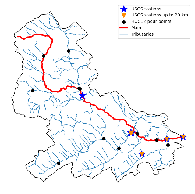
First, let’s get the watershed geometry of the contributing basin of a USGS station using NLDI:

nldi = NLDI()
station_id = "01031500"

basin = nldi.get_basins(station_id)

The navigate_byid class method can be used to navigate NHDPlus in both upstream and downstream of any point in the database. The available feature sources are comid, huc12pp, nwissite, wade, wqp. Let’s get ComIDs and flowlines of the tributaries and the main river channel in the upstream of the station.

flw_main = nldi.navigate_byid(
    fsource="nwissite",
    fid=f"USGS-{station_id}",
    navigation="upstreamMain",
    source="flowlines",
    distance=1000,
)

flw_trib = nldi.navigate_byid(
    fsource="nwissite",
    fid=f"USGS-{station_id}",
    navigation="upstreamTributaries",
    source="flowlines",
    distance=1000,
)

We can get other USGS stations upstream (or downstream) of the station and even set a distance limit (in km):

st_all = nldi.navigate_byid(
    fsource="nwissite",
    fid=f"USGS-{station_id}",
    navigation="upstreamTributaries",
    source="nwissite",
    distance=1000,
)

st_d20 = nldi.navigate_byid(
    fsource="nwissite",
    fid=f"USGS-{station_id}",
    navigation="upstreamTributaries",
    source="nwissite",
    distance=20,
)

Now, let’s get the HUC12 pour points:

pp = nldi.navigate_byid(
    fsource="nwissite",
    fid=f"USGS-{station_id}",
    navigation="upstreamTributaries",
    source="huc12pp",
    distance=1000,
)

Let’s plot the vector data:

ax = basin.plot(facecolor="none", edgecolor="k", figsize=(8, 8))
st_all.plot(ax=ax, label="USGS stations", marker="*", markersize=300, zorder=4, color="b")
st_d20.plot(
    ax=ax,
    label="USGS stations up to 20 km",
    marker="v",
    markersize=100,
    zorder=5,
    color="darkorange",
)
pp.plot(ax=ax, label="HUC12 pour points", marker="o", markersize=50, color="k", zorder=3)
flw_main.plot(ax=ax, lw=3, color="r", zorder=2, label="Main")
flw_trib.plot(ax=ax, lw=1, zorder=1, label="Tributaries")
ax.legend(loc="best")
ax.set_aspect("auto")
ax.set_axis_off()
ax.figure.set_dpi(100)
ax.figure.savefig("_static/nhdplus_navigation.png", bbox_inches="tight", facecolor="w")

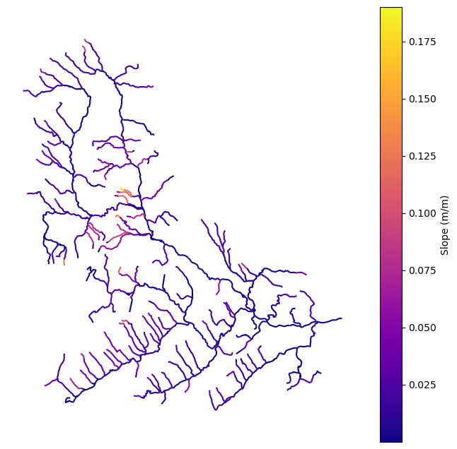
Next, we get the slope data for each river segment from NHDPlus VAA database:

vaa = nhd.nhdplus_vaa("input_data/nhdplus_vaa.parquet")

flw_trib["comid"] = pd.to_numeric(flw_trib.nhdplus_comid)
slope = gpd.GeoDataFrame(
    pd.merge(flw_trib, vaa[["comid", "slope"]], left_on="comid", right_on="comid"),
    crs=flw_trib.crs,
)
slope[slope.slope < 0] = np.nan

ax = slope.plot(
    figsize=(8, 8),
    column="slope",
    cmap="plasma",
    legend=True,
    legend_kwds={"label": "Slope (m/m)"},
)
ax.set_axis_off()

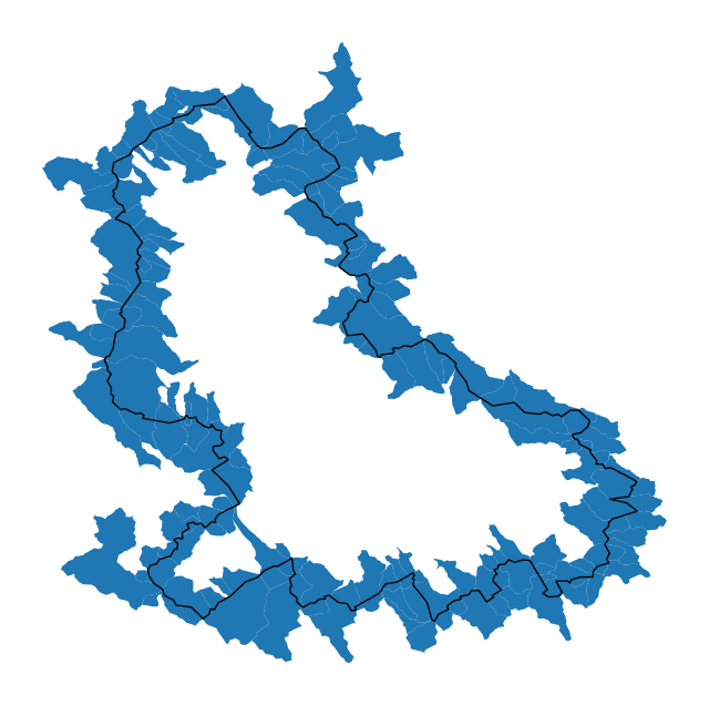
Now, let’s use WaterData service to get the headwater catchments for this basin:

wd_cat = WaterData("catchmentsp")
cat = wd_cat.bygeom(basin.geometry[0], predicate="overlaps")

ax = cat.plot(figsize=(8, 8))
basin.plot(ax=ax, facecolor="none", edgecolor="k")
ax.set_aspect("auto")
ax.figure.set_dpi(100)
ax.set_axis_off()

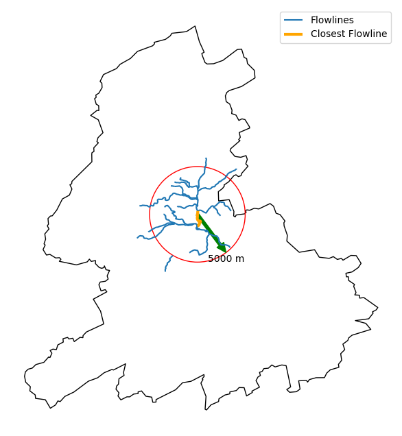
We might to get all the HUC12 pour points within a radius of an station. We can achieve this using bydistance method of WaterData class. For example, let’s take station 01031300 and find all the flowlines within a radius of 5 km.

eck4 = "+proj=eck4 +lon_0=0 +x_0=0 +y_0=0 +datum=WGS84 +units=m +no_defs"
st300 = st_all[st_all.identifier == "USGS-01031300"].to_crs(eck4)
coords = st300.geometry.values[0].coords.xy
x, y = coords[0][0], coords[1][0]
rad = 5e3

nhdp_mr = WaterData("nhdflowline_network")

flw_rad = nhdp_mr.bydistance((x, y), rad, loc_crs=eck4)
flw_rad = flw_rad.to_crs(eck4)

Instead of getting all features within a radius of the coordinate, we can snap to the closest flowline using NLDI:

comid_closest = nldi.comid_byloc((x, y), eck4)
flw_closest = nhdp_mr.byid("comid", comid_closest.comid.values[0])

ax = basin.to_crs(eck4).plot(figsize=(8, 8), facecolor="none", edgecolor="k")
flw_rad.plot(ax=ax)
flw_closest.to_crs(eck4).plot(ax=ax, color="orange", lw=3)
ax.legend(["Flowlines", "Closest Flowline"])

circle = mpatches.Circle((x, y), rad, ec="r", fill=False)
arrow = mpatches.Arrow(x, y, 0.6 * rad, -0.8 * rad, width=1500, color="g")
ax.text(x + 0.6 * rad, y + -rad, f"{int(rad)} m", ha="center")
ax.add_artist(circle)
ax.set_aspect("equal")
ax.add_artist(arrow)
ax.figure.set_dpi(100)
ax.axis("off")
ax.figure.savefig("_static/nhdplus_radius.png", bbox_inches="tight", facecolor="w")

WaterData gives us access to the medium-resolution NHDPlus database. We can use NHDPlusHR to retrieve high-resolution NHDPlus data. Let’s get both medium- and high-resolution flowlines within the bounding box of our watershed and compare them. Moreover, Since several web services offer access to NHDPlus database, NHDPlusHR has an argument for selecting a service and also an argument for automatically switching between services.

flw_mr = nhdp_mr.bybox(basin.geometry[0].bounds)

nhdp_hr = NHDPlusHR("flowline")
flw_hr = nhdp_hr.bygeom(basin.geometry[0].bounds)

fig, (ax1, ax2) = plt.subplots(1, 2, figsize=(12, 8), facecolor="w")

flw_mr.plot(ax=ax1)
ax1.set_title("NHDPlus Medium Resolution")
ax1.set_axis_off()
flw_hr.plot(ax=ax2)
ax2.set_title("NHDPlus High Resolution")
ax2.set_axis_off()
fig.savefig("_static/hr_mr.png", bbox_inches="tight", facecolor="w")

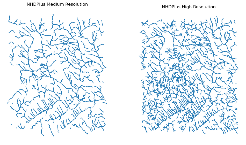
Since NHDPlus HR is still at the pre-release stage, let’s use the MR flowlines to demonstrate the vector-based accumulation.

Based on a topological sorted river network pynhd.vector_accumulation computes flow accumulation in the network. It returns a dataframe which is sorted from upstream to downstream that shows the accumulated flow in each node.

PyNHD has a utility called prepare_nhdplus that identifies such relationship among other things such as fixing some common issues with NHDPlus flowlines. But first we need to get all the NHDPlus attributes for each ComID since NLDI only provides the flowlines’ geometries and ComIDs which is useful for navigating the vector river network data. For getting the NHDPlus database we use WaterData. The WaterData web service layers are nhdflowline_network, nhdarea, nhdwaterbody, catchmentsp, gagesii, huc08, huc12, huc12agg, and huc12all. Let’s use the nhdflowline_network layer to get required info.

comids = [int(c) for c in flw_trib.nhdplus_comid.to_list()]
nhdp_trib = nhdp_mr.byid("comid", comids)
flw = nhd.prepare_nhdplus(nhdp_trib, 0, 0, purge_non_dendritic=False)

To demonstrate the use of routing, let’s use nhdplus_attrs function to get list of available NHDPlus attributes from Select Attributes for NHDPlus Version 2.1 Reach Catchments and Modified Network Routed Upstream Watersheds for the Conterminous United States item on ScienceBase service. These attributes are in catchment-scale and are available in three categories:

1. Local (local): For individual reach catchments,

2. Total (upstream_acc): For network-accumulated values using total cumulative drainage area,

3. Divergence (div_routing): For network-accumulated values using divergence-routed.

nldi.valid_characteristics.head(5)

	characteristic_id	characteristic_description	units	dataset_label	dataset_url	theme_label	theme_url	characteristic_type
0	CAT_WILDFIRE_2011	percent of wild fires per catchments for 2011	percent	Estimated percent of catchment that experience...	https://www.sciencebase.gov/catalog/item/57f66...	Land Cover	unknown	localCatch_name
1	CAT_CONTACT	Subsurface flow contact time index. The subsur...	days	Contact time, the length of time it takes for ...	https://www.sciencebase.gov/catalog/item/56f96...	Hydrologic	https://www.sciencebase.gov/catalog/item/5669a...	localCatch_name
2	CAT_EWT	Average depth to water table relatice to the l...	meters	Average depth to water table relative to land ...	https://www.sciencebase.gov/catalog/item/56f97...	Hydrologic	https://www.sciencebase.gov/catalog/item/5669a...	localCatch_name
3	CAT_FUNGICIDE	Fungicide use on agricultural land in kilogram...	kilogram per square kilometer	Fungicide use on agricultural land in kilogram...	https://www.sciencebase.gov/catalog/item/56fd6...	Chemical	https://www.sciencebase.gov/catalog/item/56fd6...	localCatch_name
4	CAT_IEOF	Percentage of Horton overland flow as a percent	percent	Mean infiltration-excess overland flow as a pe...	https://www.sciencebase.gov/catalog/item/56f97...	Hydrologic	https://www.sciencebase.gov/catalog/item/5669a...	localCatch_name

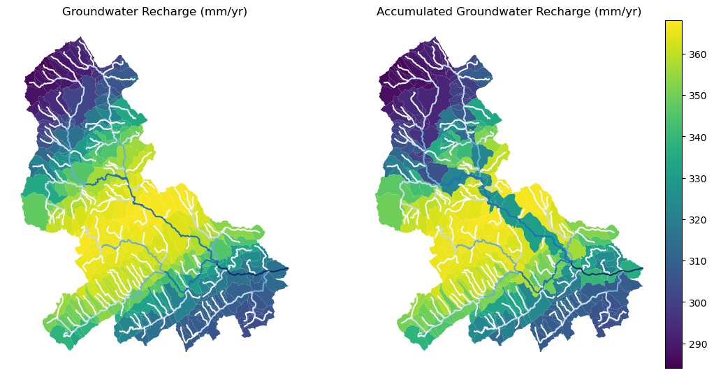
Let’s get Mean Annual Groundwater Recharge, RECHG, using getcharacteristic_byid class method and carry out the flow accumulation.

char = "CAT_RECHG"
area = "areasqkm"

local = nldi.getcharacteristic_byid(comids, "local", char_ids=char)
flw = flw.merge(local[char], left_on="comid", right_index=True)


def runoff_acc(qin, q, a):
    return qin + q * a


flw_r = flw[["comid", "tocomid", char, area]]
runoff = nhd.vector_accumulation(flw_r, runoff_acc, char, [char, area])


def area_acc(ain, a):
    return ain + a


flw_a = flw[["comid", "tocomid", area]]
areasqkm = nhd.vector_accumulation(flw_a, area_acc, area, [area])

runoff /= areasqkm

Since these are catchment-scale characteristic, let’s get the catchments then add the accumulated characteristic as a new column and plot the results.

catchments = wd_cat.byid("featureid", comids)

c_local = catchments.merge(local, left_on="featureid", right_index=True)
c_acc = catchments.merge(runoff, left_on="featureid", right_index=True)

/var/folders/jx/s06wj7hs325c_2yd2g5209sr0000gp/T/ipykernel_77507/1102694309.py:1: UserWarning: 8 of 432 requests failed.. IDs of the failed requests are ['1723523', '1723331', '1721829', '1721855', '1721857', '1723355', '1723559', '1721835']
  catchments = wd_cat.byid("featureid", comids)

fig, (ax1, ax2) = plt.subplots(1, 2, figsize=(12, 8), facecolor="w")

cmap = "viridis"
norm = plt.Normalize(vmin=c_local.CAT_RECHG.min(), vmax=c_acc.acc_CAT_RECHG.max())

c_local.plot(ax=ax1, column=char, cmap=cmap, norm=norm)
flw.plot(ax=ax1, column="streamorde", cmap="Blues", scheme="fisher_jenks")
ax1.set_title("Groundwater Recharge (mm/yr)")
ax1.set_axis_off()

c_acc.plot(ax=ax2, column=f"acc_{char}", cmap=cmap, norm=norm)
flw.plot(ax=ax2, column="streamorde", cmap="Blues", scheme="fisher_jenks")
ax2.set_title("Accumulated Groundwater Recharge (mm/yr)")
ax2.set_axis_off()

cax = fig.add_axes(
    [
        ax2.get_position().x1 + 0.01,
        ax2.get_position().y0,
        0.02,
        ax2.get_position().height,
    ]
)
sm = plt.cm.ScalarMappable(cmap=cmap, norm=norm)
fig.colorbar(sm, cax=cax)
fig.savefig(Path("_static", "flow_accumulation.png"), bbox_inches="tight", facecolor="w")